46. Spectral Element Method - Elastic Wave Equation 1D - Homogeneous Case#
This notebook covers the following aspects:
The weak form of the 1D elastic wave equation
Initialization and implementataion of the Mass and Stiffness Matrices
Solution using the finite difference scheme and its comparion with FEM solution
46.1. Basic Equations#
This notebook presents the numerical solution for the 1D elastic wave equation
\begin{equation} \rho(x) \partial_t^2 u(x,t) = \partial_x (\mu(x) \partial_x u(x,t)) + f(x,t), \end{equation}
using the spectral element method. This is done after a series of steps summarized as follow:
The wave equation is written into its weak form
Assume stress-free boundary condition after integration by parts
Approximate the wave field as a linear combination of some basis
\begin{equation} u(x,t) \ \approx \ \overline{u}(x,t) \ = \ \sum_{i=1}^{n} u_i(t) \ \varphi_i(x) \end{equation}
Use the same basis functions in \(u(x, t)\) as test functions in the weak form, the so call Galerkin principle.
The continuous weak form is written as a system of linear equations by considering the approximated displacement field.
\begin{equation} \mathbf{M}^T\partial_t^2 \mathbf{u} + \mathbf{K}^T\mathbf{u} = \mathbf{f} \end{equation}
Time extrapolation with centered finite differences scheme
\begin{equation} \mathbf{u}(t + dt) = dt^2 (\mathbf{M}^T)^{-1}[\mathbf{f} - \mathbf{K}^T\mathbf{u}] + 2\mathbf{u} - \mathbf{u}(t-dt). \end{equation}
where \(\mathbf{M}\) is known as the mass matrix, and \(\mathbf{K}\) the stiffness matrix.
The above solution is exactly the same presented for the classic finite-element method. Now we introduce appropriated basis functions and integration scheme to efficiently solve the system of matrices.
46.1.1. Interpolation with Lagrange Polynomials#
At the elemental level, we introduce as interpolating functions the Lagrange polynomials and use \(\xi\) as the space variable representing our elemental domain:
\begin{equation}
\varphi_i \ \rightarrow \ \ell_i^{(N)} (\xi) \ := \ \prod_{j \neq i}^{N+1} \frac{\xi - \xi_j}{\xi_i-\xi_j}, \qquad i,j = 1, 2, \dotsc , N + 1
\end{equation}
46.1.2. Numerical Integration#
The integral of a continuous function \(f(x)\) can be calculated after replacing \(f(x)\) by a polynomial approximation that can be integrated analytically. As interpolating functions we use again the Lagrange polynomials and obtain Gauss-Lobatto-Legendre quadrature. Here, the GLL points are used to perform the integral.
\begin{equation} \int_{-1}^1 f(x) \ dx \approx \int {-1}^1 P_N(x) dx = \sum{i=1}^{N+1} w_i f(x_i) \end{equation}
import matplotlib.pyplot as plt
import numpy as np
from gll import gll
from lagrange1st import lagrange1st
from ricker import ricker
# Show Plot in The Notebook
# matplotlib.use("nbagg")
46.1.3. 1. Initialization of setup#
# Initialization of setup
# ---------------------------------------------------------------
nt = 600  # number of time steps
xmax = 10000.0  # Length of domain [m]
vs = 2500.0  # S velocity [m/s]
rho = 2000  # Density [kg/m^3]
mu = rho * vs**2  # Shear modulus mu
N = 5  # Order of Lagrange polynomials
ne = 125  # Number of elements
Tdom = 0.1  # Dominant period of Ricker source wavelet
iplot = 5  # Plotting each iplot snapshot

# variables for elemental matrices
Me = np.zeros(N + 1, dtype=float)
Ke = np.zeros((N + 1, N + 1), dtype=float)
# ----------------------------------------------------------------

# Initialization of GLL points integration weights
[xi, w] = gll(N)  # xi, N+1 coordinates [-1 1] of GLL points
# w Integration weights at GLL locations
# Space domain
le = xmax / ne  # Length of elements
# Vector with GLL points
k = 0

# Initialization of physical coordinates xg in the entire space (commment added May 15, 2020)
xg = np.zeros((N * ne) + 1)
xg[k] = 0
for i in range(1, ne + 1):
    for j in range(0, N):
        k = k + 1
        xg[k] = (i - 1) * le + 0.5 * (xi[j + 1] + 1) * le

# ---------------------------------------------------------------
dxmin = min(np.diff(xg))
eps = 0.2  # Courant value
dt = eps * dxmin / vs  # Global time step

# Mapping - Jacobian
J = le / 2
Ji = 1 / J  # Inverse Jacobian

# 1st derivative of Lagrange polynomials
l1d = lagrange1st(N)  # Array with GLL as columns for each N+1 polynomial
46.1.4. 2. The Mass Matrix#
Now we initialize the mass and stiffness matrices. In general, the mass matrix at the elemental level is given
\begin{equation} M_{ji}^e \ = \ w_j \ \rho (\xi) \ \frac{\mathrm{d}x}{\mathrm{d}\xi} \delta_{ij} \vert_ {\xi = \xi_j} \end{equation}
We implement the mass matrix using the integration weights at GLL locations \(w\), the jacobian \(J\), and density \(\rho\). Then, perform the global assembly of the mass matrix, compute its inverse, and display the inverse mass matrix to visually inspect how it looks like.
# Elemental Mass matrix
# ---------------------------------------------------------------
for i in range(0, N + 1):
    Me[i] = rho * w[i] * J  # stored as a vector since it's diagonal

# Global Mass matrix
# ---------------------------------------------------------------
k = -1
ng = (ne - 1) * N + N + 1
M = np.zeros(2 * ng)

for i in range(1, ne + 1):
    for j in range(0, N + 1):
        k = k + 1
        if i > 1:
            if j == 0:
                k = k - 1
        M[k] = M[k] + Me[j]

# Inverse matrix of M
# ---------------------------------------------------------------
Minv = np.identity(ng)
for i in range(0, ng):
    Minv[i, i] = 1.0 / M[i]

# --------------------------------------------------------------
# Display inverse mass matrix inv(M)
# --------------------------------------------------------------
plt.imshow(Minv)
plt.title(r"Mass Matrix $\mathbf{M}$")
plt.axis("off")
plt.tight_layout()
plt.show()

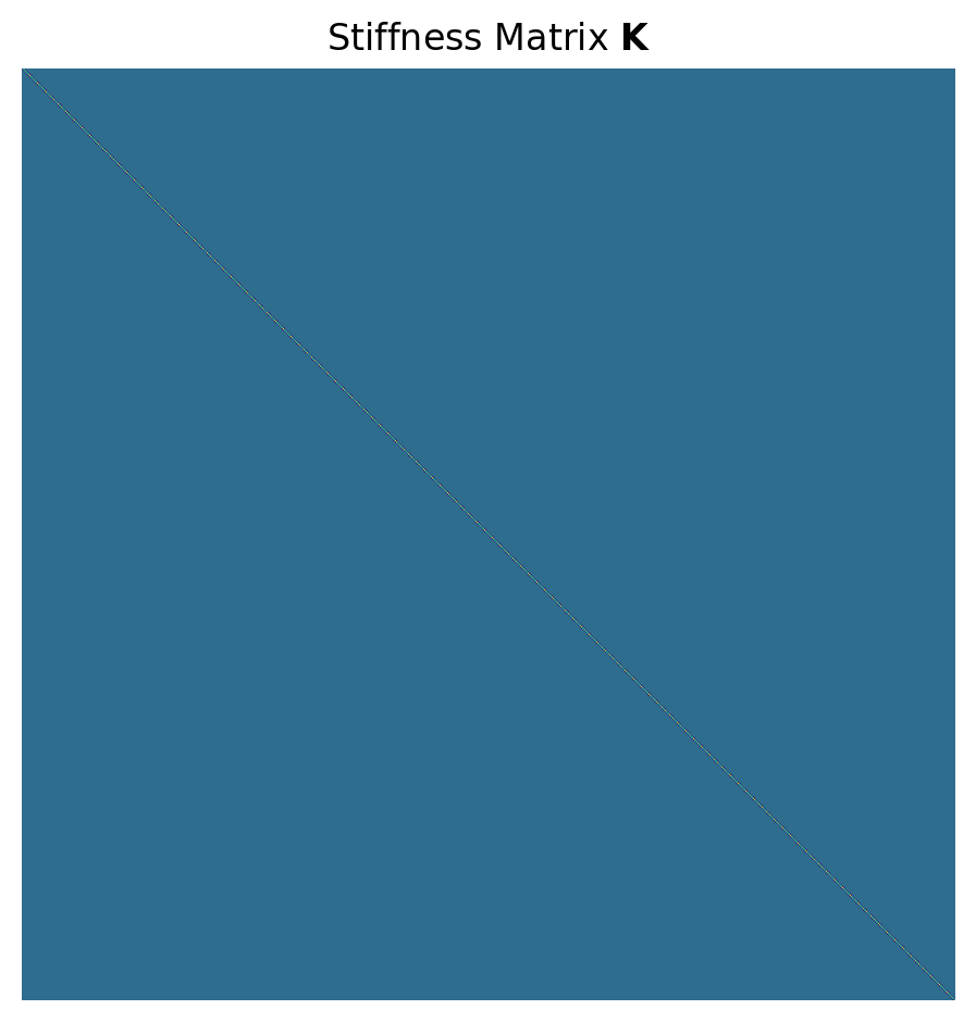
46.1.5. 3. The Stiffness matrix#
On the other hand, the general form of the stiffness matrix at the elemtal level is
\begin{equation} K_{ji}^e \ = \ \sum_{k = 1}^{N+1} w_k \mu (\xi) \partial_\xi \ell_j (\xi) \partial_\xi \ell_i (\xi) \left(\frac{\mathrm{d}\xi}{\mathrm{d}x} \right)^2 \frac{\mathrm{d}x}{\mathrm{d}\xi} \vert_{\xi = \xi_k} \end{equation}
We implement the stiffness matrix using the integration weights at GLL locations \(w\), the jacobian \(J\), and shear stress \(\mu\). Then, perform the global assembly of the mass matrix and display the matrix to visually inspect how it looks like.
# Elemental Stiffness Matrix
# ---------------------------------------------------------------
for i in range(0, N + 1):
    for j in range(0, N + 1):
        for k in range(0, N + 1):
            Ke[i, j] = Ke[i, j] + mu * w[k] * Ji * l1d[i, k] * l1d[j, k]

# Global Stiffness Matrix
# ---------------------------------------------------------------
K = np.zeros([ng, ng])
# Values except at element boundaries
for k in range(1, ne + 1):
    i0 = (k - 1) * N + 1
    j0 = i0
    for i in range(-1, N):
        for j in range(-1, N):
            K[i0 + i, j0 + j] = Ke[i + 1, j + 1]

# Values at element boundaries
for k in range(2, ne + 1):
    i0 = (k - 1) * N
    j0 = i0
    K[i0, j0] = Ke[0, 0] + Ke[N, N]


# --------------------------------------------------------------
# Display stiffness matrix K
# --------------------------------------------------------------
plt.imshow(K)
plt.title(r"Stiffness Matrix $\mathbf{K}$")
plt.axis("off")

plt.tight_layout()
plt.show()
46.1.6. 4. Spectral Element solution#
Finally we implement the spectral element solution using the computed mass \(M\) and stiffness \(K\) matrices together with a finite differences extrapolation scheme
\begin{equation} \mathbf{u}(t + dt) = dt^2 (\mathbf{M}^T)^{-1}[\mathbf{f} - \mathbf{K}^T\mathbf{u}] + 2\mathbf{u} - \mathbf{u}(t-dt). \end{equation}
# SE Solution, Time extrapolation
# ---------------------------------------------------------------
# initialize source time function and force vector f
src = ricker(dt, Tdom)
isrc = int(np.floor(ng / 2)) # Source location
# Initialization of solution vectors
u = np.zeros(ng)
uold = u
unew = u
f = u
# --------------------------------------------------------------
# Initialize animated plot
# --------------------------------------------------------------
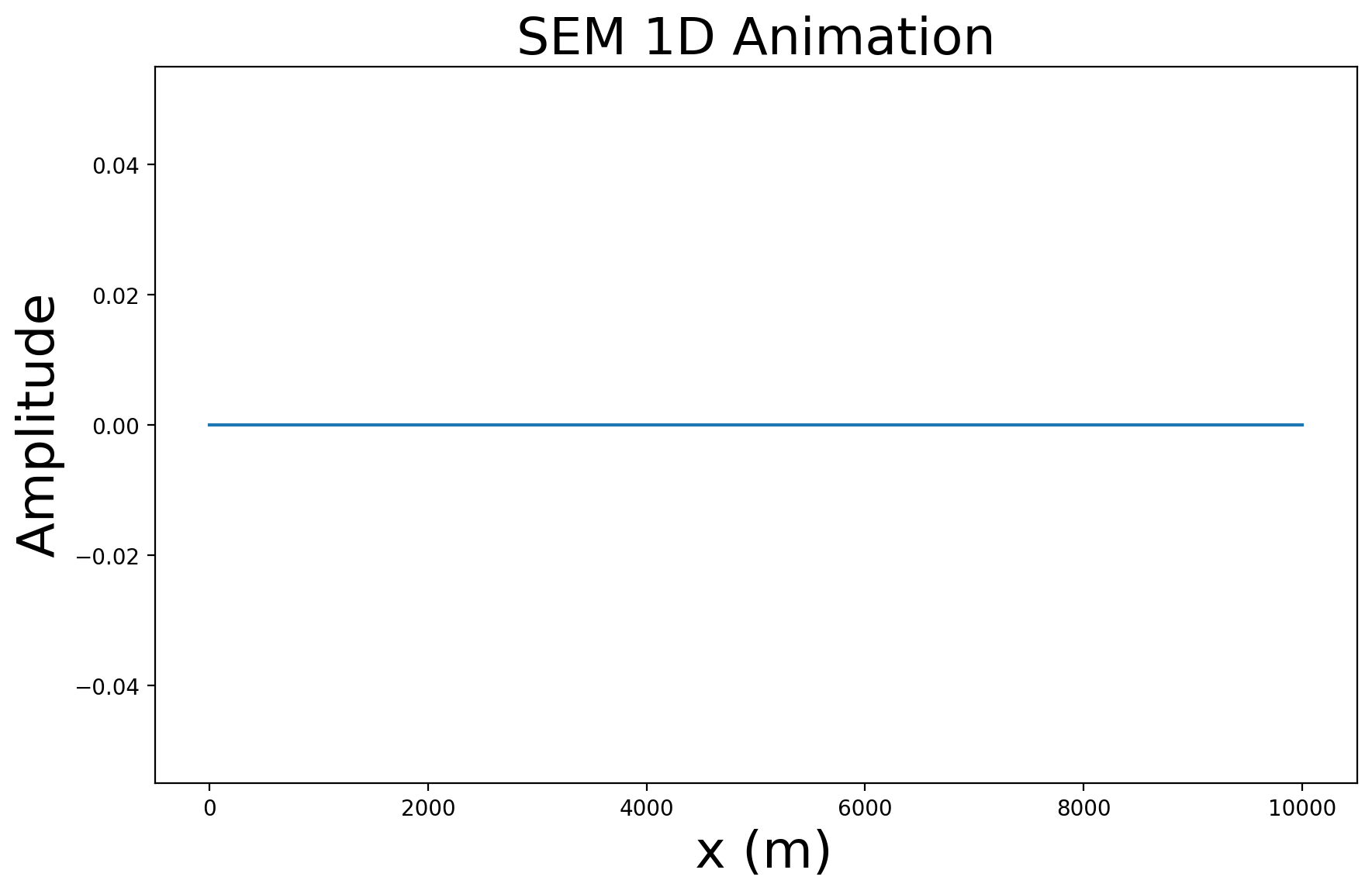
plt.figure(figsize=(10, 6))
lines = plt.plot(xg, u, lw=1.5)
plt.title("SEM 1D Animation", size=24)
plt.xlabel(" x (m)", size=24)
plt.ylabel(" Amplitude ", size=24)
plt.rc("xtick", labelsize=20) # fontsize of the tick labels
plt.rc("ytick", labelsize=20) # fontsize of the tick labels
plt.ion() # set interective mode
plt.show()
# ---------------------------------------------------------------
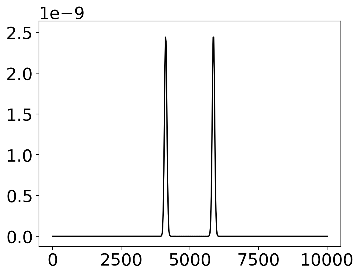
# Time extrapolation
# ---------------------------------------------------------------
for it in range(nt):
# Source initialization
f = np.zeros(ng)
if it < len(src):
f[isrc - 1] = src[it - 1]
# Time extrapolation
unew = dt**2 * Minv @ (f - K @ u) + 2 * u - uold
uold, u = u, unew
# --------------------------------------
# Animation plot. Display solution
if not it % iplot:
for l in lines:
l.remove()
del l
# --------------------------------------
# Display lines
lines = plt.plot(xg, u, color="black", lw=1.5)
plt.gcf().canvas.draw()