16. 1D heat diffusion

Uses the Python interface to PETSc (petsc4py) to solve the transient 1D heat
diffusion with Dirichlet Boundary Conditions. This is a super simple example
showcase of the linear iterative solvers PETSc has to offer. It runs
sequentially without MPI.

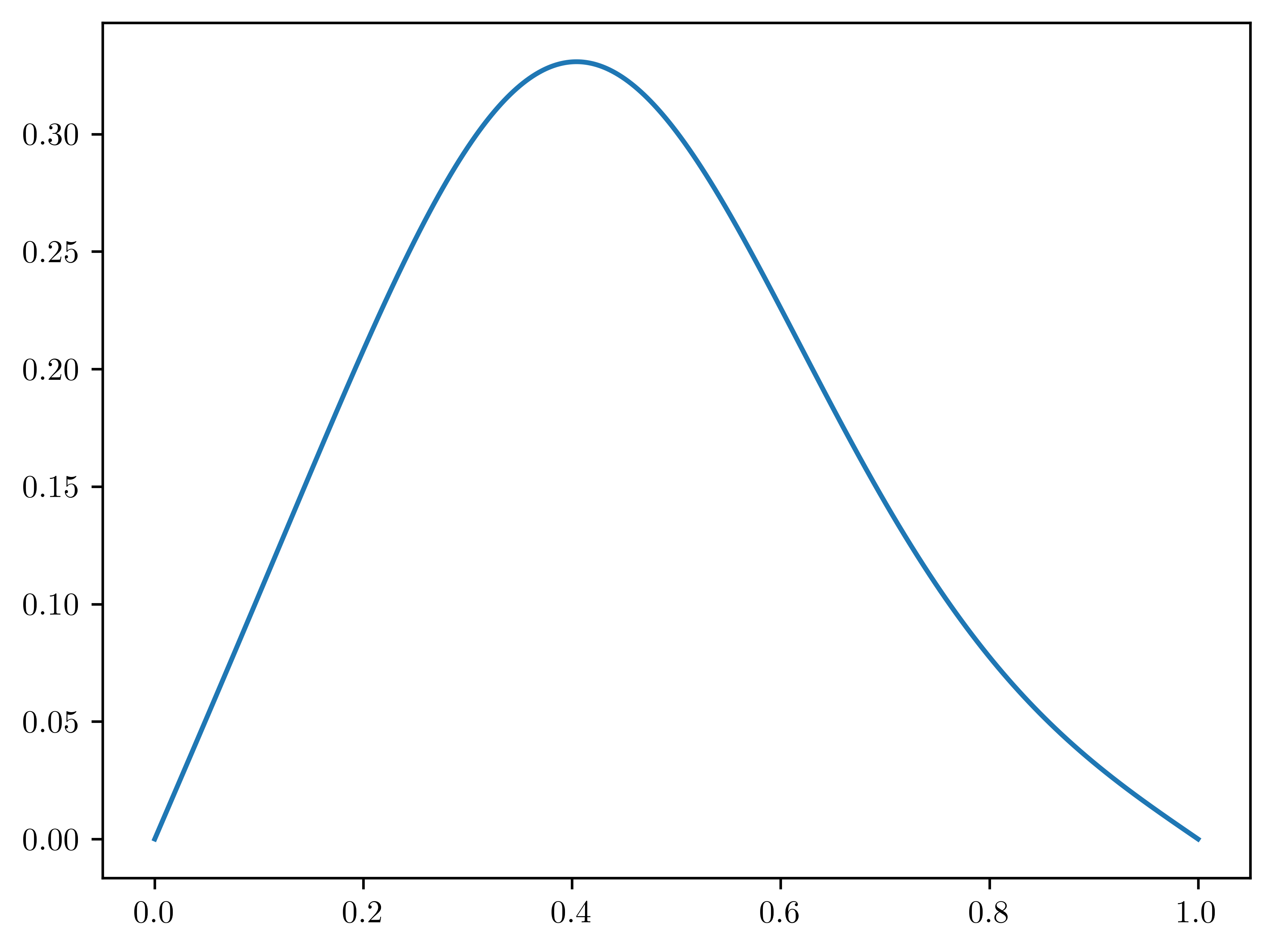
Consider the 1D heat equation defining how a temperature is distributed e.g.
over a one-dimensional rod.

    ∂u/∂t = ∂²u/∂x²

with Dirichlet Boundary Conditions at both ends of a unit domain

    u(t, x=0) = 0 = u(t, x=1)

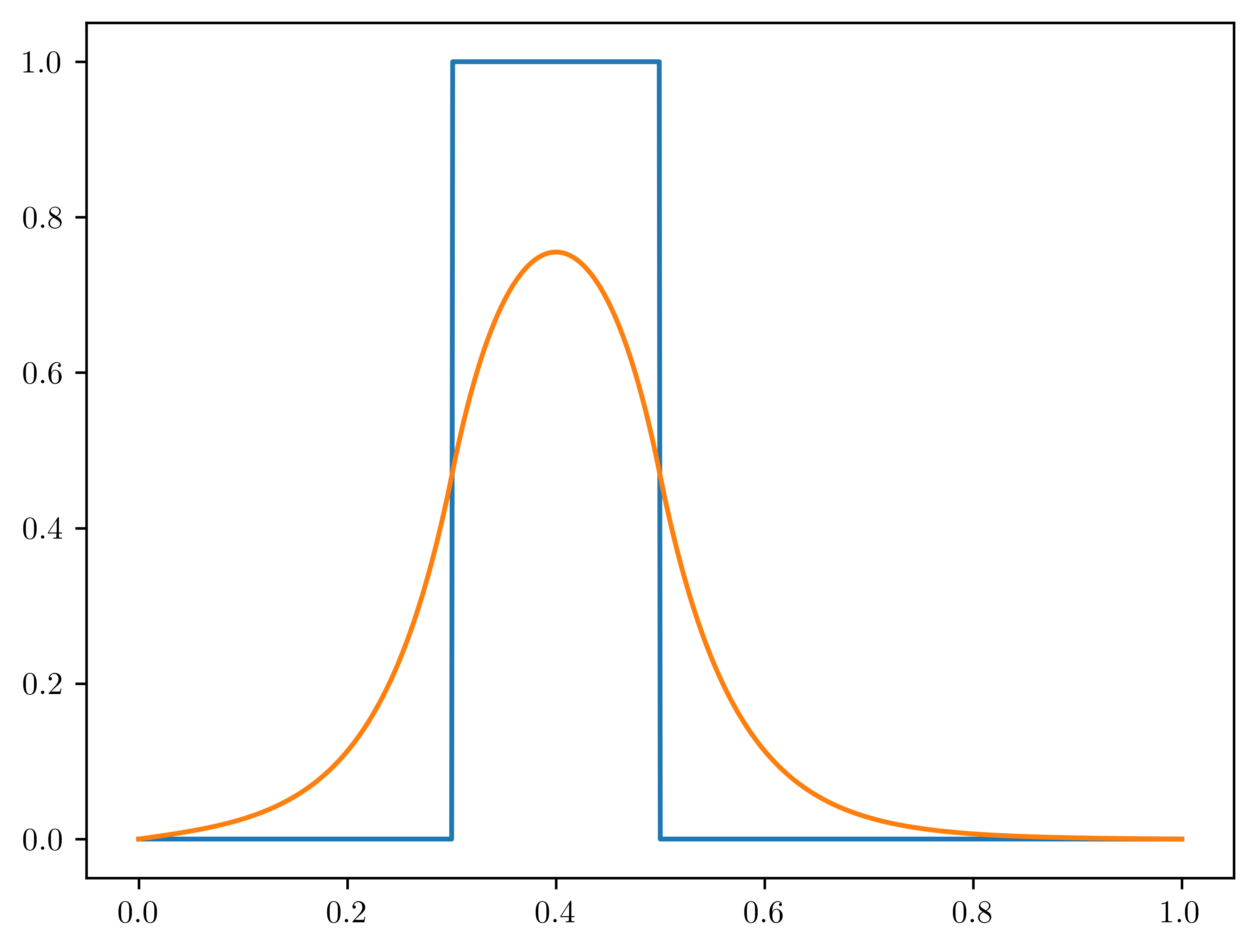
and the following initial condition

         ┌────────────────────────────────────────┐   
         │⢸⠀⠀⠀⠀⠀⠀⠀⠀⠀⠀⠀⢰⠒⠒⠒⠒⠒⠒⢲⠀⠀⠀⠀⠀⠀⠀⠀⠀⠀⠀⠀ │ y1
         │⢸⠀⠀⠀⠀⠀⠀⠀⠀⠀⠀⠀⢸⠀⠀⠀⠀⠀⠀⢸⠀⠀⠀⠀⠀⠀⠀⠀⠀⠀⠀ ⠀│   
         │⢸⠀⠀⠀⠀⠀⠀⠀⠀⠀⠀⠀⢸⠀⠀⠀⠀⠀⠀⢸⠀⠀⠀⠀⠀⠀⠀⠀⠀⠀⠀ ⠀│   
         │⢸⠀⠀⠀⠀⠀⠀⠀⠀⠀⠀⠀⢸⠀⠀⠀⠀⠀⠀⢸⠀⠀⠀⠀⠀⠀⠀⠀⠀⠀⠀ ⠀│   
         │⢸⠀⠀⠀⠀⠀⠀⠀⠀⠀⠀⠀⢸⠀⠀⠀⠀⠀⠀⢸⠀⠀⠀⠀⠀⠀⠀⠀⠀⠀⠀ ⠀│   
         │⢸⠀⠀⠀⠀⠀⠀⠀⠀⠀⠀⠀⢸⠀⠀⠀⠀⠀⠀⢸⠀⠀⠀⠀⠀⠀⠀⠀⠀⠀⠀ ⠀│   
         │⢸⠀⠀⠀⠀⠀⠀⠀⠀⠀⠀⠀⢸⠀⠀⠀⠀⠀⠀⢸⠀⠀⠀⠀⠀⠀⠀⠀⠀⠀⠀ ⠀│   
         │⢸⠀⠀⠀⠀⠀⠀⠀⠀⠀⠀⠀⢸⠀⠀⠀⠀⠀⠀⢸⠀⠀⠀⠀⠀⠀⠀⠀⠀⠀⠀ ⠀│   
         │⢸⠀⠀⠀⠀⠀⠀⠀⠀⠀⠀⠀⢸⠀⠀⠀⠀⠀⠀⢸⠀⠀⠀⠀⠀⠀⠀⠀⠀⠀⠀ ⠀│   
         │⢸⠀⠀⠀⠀⠀⠀⠀⠀⠀⠀⠀⢸⠀⠀⠀⠀⠀⠀⢸⠀⠀⠀⠀⠀⠀⠀⠀⠀⠀⠀ ⠀│   
         │⢸⠀⠀⠀⠀⠀⠀⠀⠀⠀⠀⠀⢸⠀⠀⠀⠀⠀⠀⢸⠀⠀⠀⠀⠀⠀⠀⠀⠀⠀⠀ ⠀│   
         │⢸⠀⠀⠀⠀⠀⠀⠀⠀⠀⠀⠀⢸⠀⠀⠀⠀⠀⠀⢸⠀⠀⠀⠀⠀⠀⠀⠀⠀⠀⠀ ⠀│   
         │⢸⠀⠀⠀⠀⠀⠀⠀⠀⠀⠀⠀⡸⠀⠀⠀⠀⠀⠀⢸⠀⠀⠀⠀⠀⠀⠀⠀⠀⠀⠀ ⠀│   
         │⢸⠀⠀⠀⠀⠀⠀⠀⠀⠀⠀⠀⡇⠀⠀⠀⠀⠀⠀⢸⠀⠀⠀⠀⠀⠀⠀⠀⠀⠀⠀ ⠀│   
         │⢼⠤⠤⠤⠤⠤⠤⠤⠤⠤⠤⠤⠧⠤⠤⠤⠤⠤⠤⠼⠤⠤⠤⠤⠤⠤⠤⠤⠤⠤⠤⠤⠤│   
         └────────────────────────────────────────┘   
          0.0                                   1.0

-----

Solution strategy (BTCS):

Denote with û the solution at the next point in time. Then use
Finite Difference discretization on a uniform mesh. Discretize
the time derivative by implicit Euler and the second spatial
derivative by central differences.

    (û[i] − u[i])/Δt = (û[i−1] − 2 û[i] + û[i+1])/Δx²

with the conditions on the Dirichlet Boundary points

    û[0] = 0.0

    û[-1] = 0.0

Move all points at next time step to the lhs and all terms at
previous time step to rhs.

    û[i] + Δt/Δx² (− û[i−1] + 2 û[i] − û[i+1]) = u[i]

This can be expressed as a linear system of equations

    A x = b

with A being

    +-----                                                ------+
    |   1.0                                                     |
    | −Δt/Δx²  1 + 2Δt/Δx²  −Δt/Δx²                             |
    |           −Δt/Δx²  1 + 2Δt/Δx²  −Δt/Δx²
A = |                       −Δt/Δx²  1 + 2Δt/Δx²  −Δt/Δx²
    |                           ⋱         ⋱         ⋱
    |                             ⋱         ⋱         ⋱
    |                            −Δt/Δx²  1 + 2Δt/Δx²  −Δt/Δx²  |
    |                                                    1.0    |
    +-----                                                ------+

A therefore has the following sparsity structure

    +---------------+
    |*              |
    |* * *          |
    |  * * *        |
A = |    * * *      |
    |      * * *    |
    |        * * *  |
    |          * * *|
    |              *|
    +---------------+

which is not fully tri-diagonal, because we did not eliminate the
Dirichlet DoF. Hence, it is also not symmetric.

-----

The PETSc linear solver can be set at runtime.

Use this command to monitor the solution process:

    python petsc_python_simple_heat_diffusion.py -ksp_monitor

Use this flag to swap the linear solver

    python petsc_python_simple_heat_diffusion.py -ksp_type [SOLVER_NAME]

from petsc4py import PETSc, init
import sys
import numpy as np
import matplotlib.pyplot as plt

[45f1bc1db132:04391] shmem: mmap: an error occurred while determining whether or not /tmp/ompi.45f1bc1db132.33333/jf.0/208076800/shared_mem_cuda_pool.45f1bc1db132 could be created.
[45f1bc1db132:04391] create_and_attach: unable to create shared memory BTL coordinating structure :: size 134217728 

init(sys.argv)

N_POINTS = 1001
TIME_STEP_LENGTH = 0.005
N_TIME_STEPS = 10

def main():
    element_length = 1.0 / (N_POINTS - 1)
    mesh = np.linspace(0.0, 1.0, N_POINTS)

    # Create a new sparse PETSc matrix, fill it and then assemble it
    A = PETSc.Mat().createAIJ([N_POINTS, N_POINTS])
    A.setUp()

    diagonal_entry = 1.0 + 2.0 * TIME_STEP_LENGTH / element_length**2
    off_diagonal_entry = - 1.0 * TIME_STEP_LENGTH / element_length**2

    A.setValue(0, 0, 1.0)
    A.setValue(N_POINTS-1, N_POINTS-1, 1.0)

    for i in range(1, N_POINTS - 1):
        A.setValue(i, i, diagonal_entry)
        A.setValue(i, i-1, off_diagonal_entry)
        A.setValue(i, i+1, off_diagonal_entry)
    
    A.assemble()

    # Define the initial condition
    initial_condition = np.where(
        (mesh > 0.3) & (mesh < 0.5),
        1.0,
        0.0,
    )

    # Assemble the initial rhs to the linear system
    b = PETSc.Vec().createSeq(N_POINTS)
    b.setArray(initial_condition)
    b.setValue(0, 0.0)
    b.setValue(N_POINTS-1, 0.0)

    # Allocate a PETSc vector storing the solution to the linear system
    x = PETSc.Vec().createSeq(N_POINTS)

    # Instantiate a linear solver: Krylow subspace linear iterative solver
    ksp = PETSc.KSP().create()
    ksp.setOperators(A)
    ksp.setFromOptions()

    chosen_solver = ksp.getType()
    print(f"Solving with {chosen_solver:}")

    plt.plot(mesh, initial_condition)
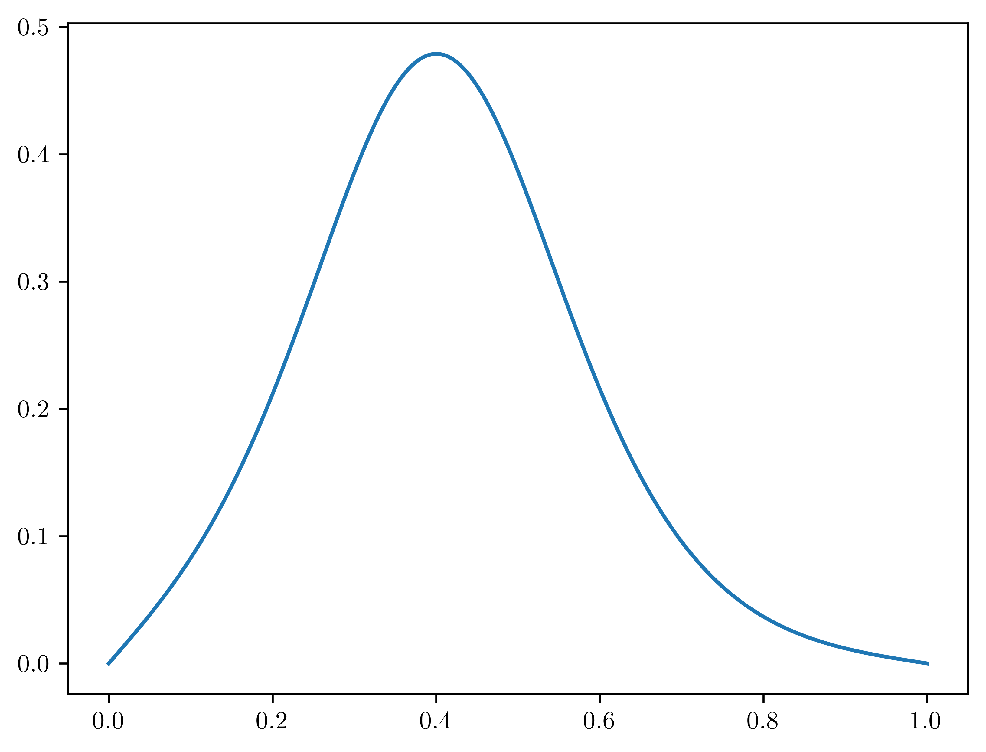
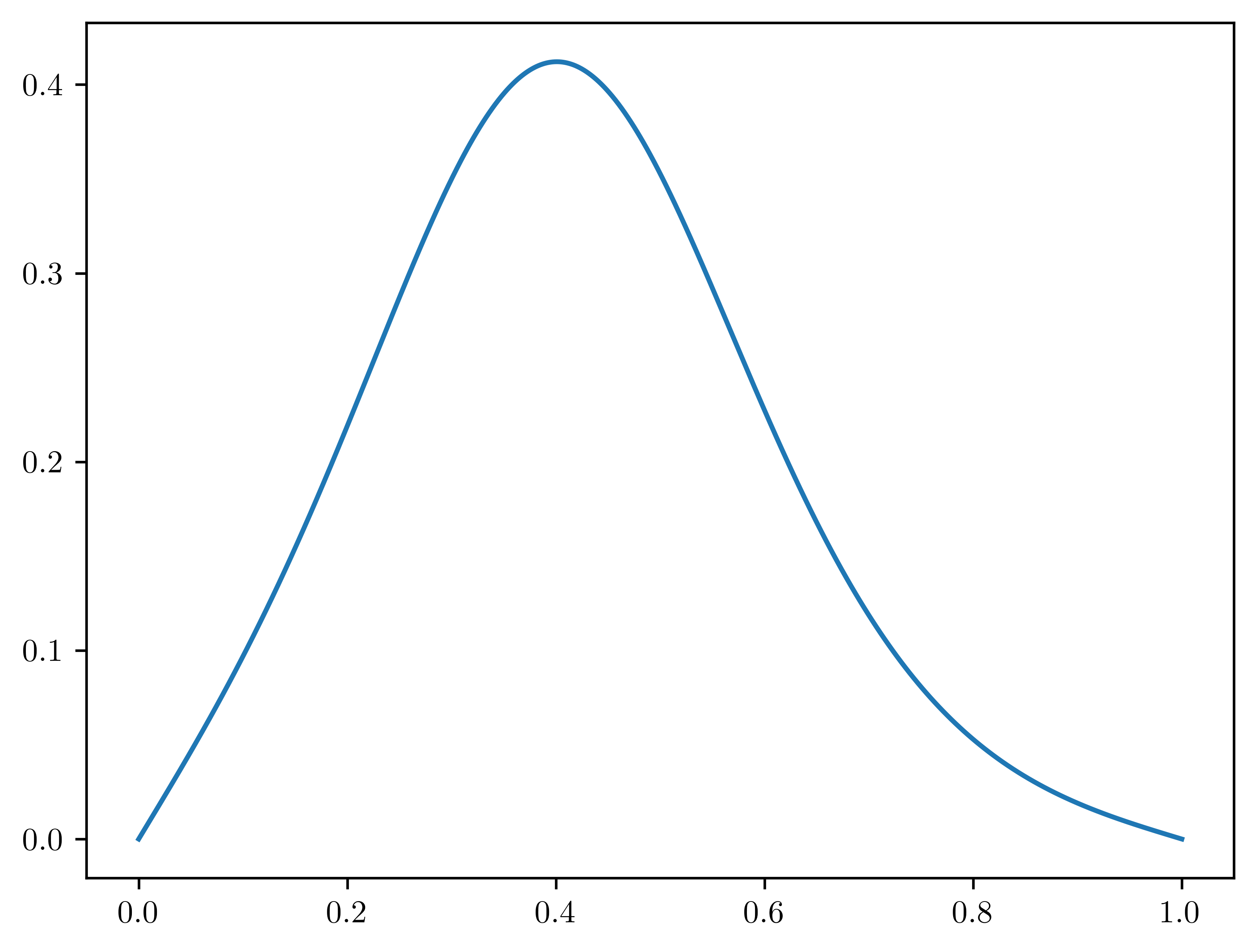
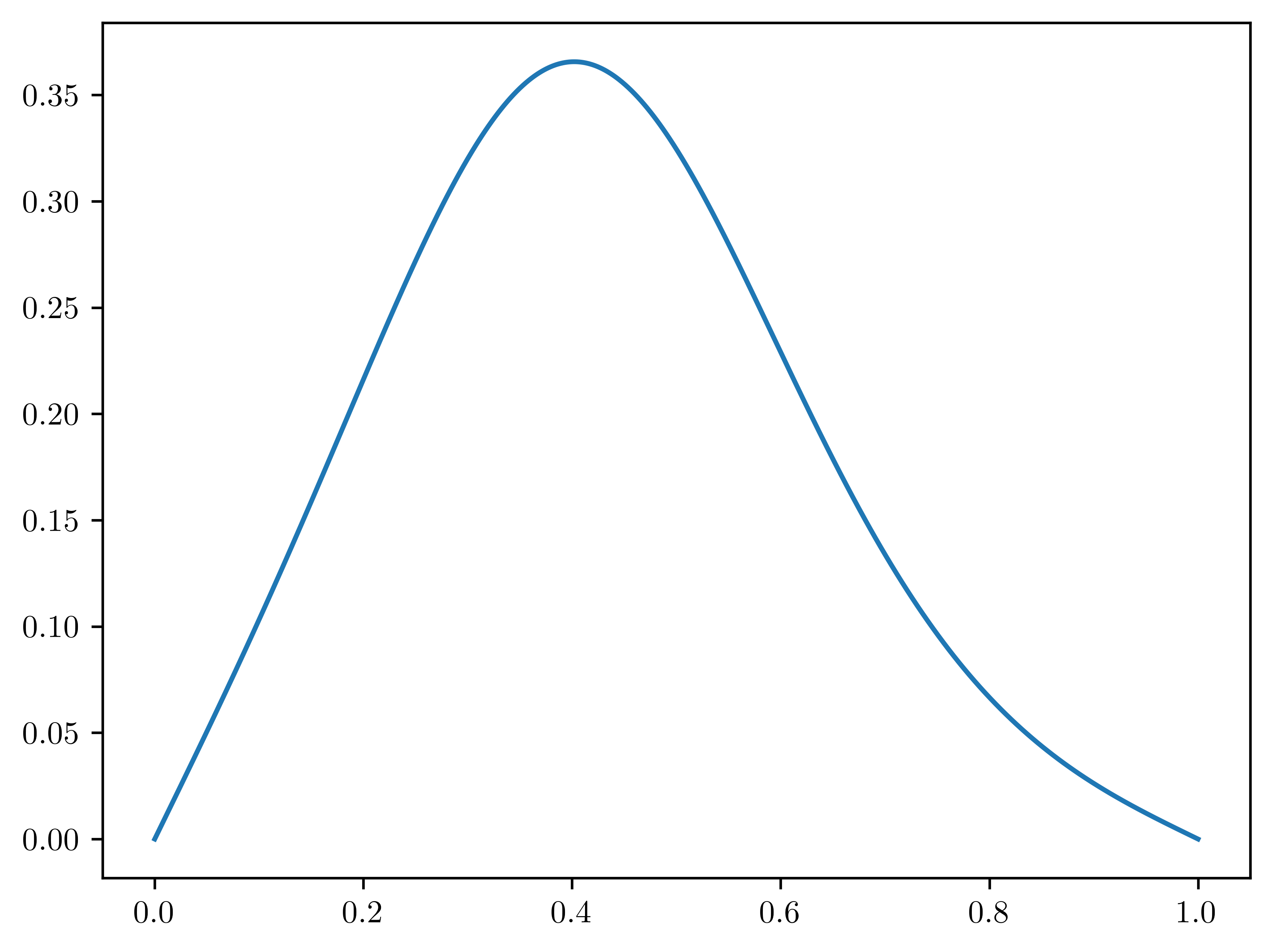
    for iter in range(N_TIME_STEPS):
        ksp.solve(b, x)

        # Re-assemble the rhs to move forward in time
        current_solution = x.getArray()
        b.setArray(current_solution)
        b.setValue(0, 0.0)
        b.setValue(N_POINTS - 1, 0.0)

        # Visualize
        plt.plot(mesh, current_solution)
        plt.draw()
        plt.pause(0.5)

    plt.show()

main()

Solving with gmres