The Pseudo-Spectral Method - Acoustic Waves in 2D

40. The Pseudo-Spectral Method - Acoustic Waves in 2D#

This notebook covers the following aspects:

Present a Fourier Pseudospectral code for solving the 2D acoustic wave equation
Compute the same using using finite difference scheme
Analyze the disperion behaviour in each case

40.1. Basic Equations#

This notebook presents a Fourier Pseudospectral code for solving the 2D acoustic wave equation. Additionally, a solution using finite difference scheme is given for comparison.

The problem of solving the wave equation

\begin{equation} \partial_t^2 p = c^2 (\partial_{x}^{2}p + \partial_{z}^{2}p) + s \end{equation}

can be achieved using finite differeces in combination with spectral methods. Here, spatial partial derivatives with respect to $x$ and $z$ are computed via the Fourier method, i.e.

\begin{equation} \partial_{x}^{2}p + \partial_{z}^{2}p = \mathscr{F}^{-1}[-k_{x}^{2}\mathscr{F}[p]] + \mathscr{F}^{-1}[-k_{z}^{2}\mathscr{F}[p]] \end{equation}

where $F$ represents the Fourier transform operator.

As it was the case in previous numerical solutions, we use a standard 3-point finite-difference operator to approximate the time derivatives. Then, the pressure field is extrapolated as

\begin{equation} \frac{p_{j,k}^{n+1} - 2p_{j,k}^{n} + p_{j,k}^{n-1}}{dt^2}= c_{j,k}^{2} (\partial_{x}^{2}p + \partial_{z}^{2}p){j,k} + s{j,k}^{n} \end{equation}

import matplotlib.pyplot as plt
import numpy as np
from ricker import ricker

# Show Plot in The Notebook
# matplotlib.use("nbagg")

40.1.1. 1. Fourier derivative method#

def fourier_derivative_2nd(f, dx):
    # Length of vector f
    nx = np.size(f)
    # Initialize k vector up to Nyquist wavenumber
    kmax = np.pi / dx
    dk = kmax / (nx / 2)
    k = np.arange(float(nx))
    k[: int(nx / 2)] = k[: int(nx / 2)] * dk
    k[int(nx / 2) :] = k[: int(nx / 2)] - kmax

    # Fourier derivative
    ff = np.fft.fft(f)
    ff = (1j * k) ** 2 * ff
    df_num = np.real(np.fft.ifft(ff))
    return df_num

40.1.2. 2. Initialization of setup#

# Basic parameters
# ---------------------------------------------------------------
nt = 600  # number of time steps
nx = 256  # number of grid points in x
nz = nx  # number of grid points in z
c = 343.0  # acoustic velocity
eps = 0.2  # stability limit
isnap = 600  # snapshot frequency
isx = int(nx / 2)  # source location
isz = int(nz / 2)
f0 = 200.0  # Frequency (div by 5)
xmax = 200
iplot = 20

# initialization of pressure fields
ap = np.zeros((nx, nz), dtype=float)
apnew = np.zeros((nx, nz), dtype=float)
apold = np.zeros((nx, nz), dtype=float)
ad2px = np.zeros((nx, nz), dtype=float)
ad2pz = np.zeros((nx, nz), dtype=float)

sp = np.zeros((nx, nz), dtype=float)
spnew = np.zeros((nx, nz), dtype=float)
spold = np.zeros((nx, nz), dtype=float)
sd2px = np.zeros((nx, nz), dtype=float)
sd2pz = np.zeros((nx, nz), dtype=float)

sp_sec = -np.abs(sp[1 : int(nx / 2), 1 : int(nz / 2)])
ap_sec = -np.abs(ap[int(nx / 2) : nx, 1 : int(nz / 2)].T)

dx = xmax / (nx - 1)  # calculate space increment
x = np.arange(0, nx) * dx  # initialize space coordinates
z = np.arange(0, nx) * dx  # initialize space coordinates
dt = eps * dx / c  # calculate tim step from stability criterion

40.1.3. 3. Source Initialization#

# source time function
# ---------------------------------------------------------------
t = np.arange(1, nt + 1) * dt  # initialize time axis
T0 = 1.0 / f0
tmp = ricker(dt, T0)
tmp = np.diff(tmp)
src = np.zeros(nt)
src[0 : np.size(tmp)] = tmp
lam = c * T0

# spatial source function
# ---------------------------------------------------------------
sg = np.zeros((nx, nz), dtype=float)
sigma = 1.5 * dx
x0 = x[isx - 1]
z0 = z[isz - 1]
for i in range(nx):
    for j in range(nz):
        sg[i, j] = np.exp(-1 / sigma**2 * ((x[i] - x0) ** 2 + (z[j] - z0) ** 2))

sg = sg / np.amax(sg)

40.1.4. 4. Time Extrapolation#

The final solution for our 2D acoustic wave problem after taking into account the finite differences time extrapolation can be written as

\begin{equation} p_{j,k}^{n+1} = dt^2c_{j,k}^{2} (\partial_{x}^{2}p + \partial_{z}^{2}p){j,k} + dt^2s{j,k}^{n} + 2p_{j,k}^{n} - p_{j,k}^{n-1} \end{equation}

In order to compare the above numerical solution, we implement a 5-point finite difference operator to compute spatial derivatives

\begin{equation} \partial_t^2 p(x,t) = \frac{-p(x,t+2\mathrm{d}t) + 16p(x,t+\mathrm{d}t) - 30p(x,t) + 16p(x,t-\mathrm{d}t) - p(x,t-2\mathrm{d}t)}{12\mathrm{d}t^2} \end{equation}

temporal derivative is done with a 3-point finite difference operator.

40.1.4.1. Numerical dispersion and anysotropy#

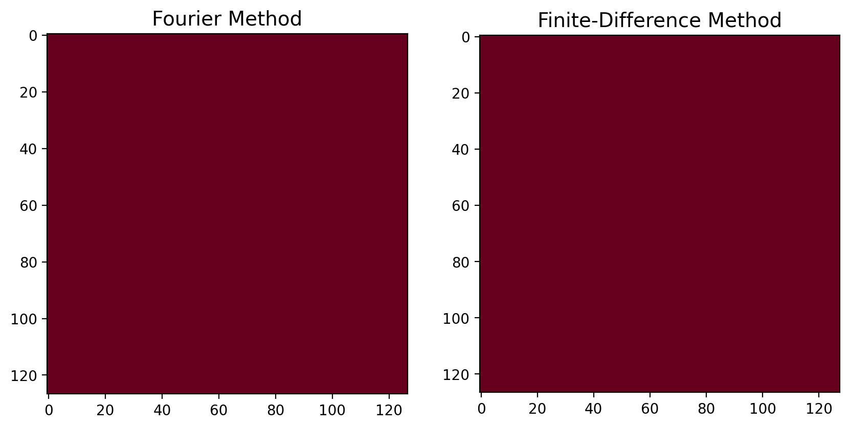
One of the most significant characteristics of the fourier method is the low numerical dispersion in comparison with the finite difference method. The snapshots displayed below for both solutions allow us to brifly comment two significant observations:

There is strong anisotropic dispersion behaviour visible for the finite-difference solution. The most accurate direction occur at $θ = π / 4$
The Fourier solution do not exhibit significant dispersion, but the most importantly, it does not seem to be directionally dependent. In other words the error is isotropic.

# Initialize animated plot
# ---------------------------------------------------------------
fig = plt.figure(figsize=(10, 6))
ax1 = fig.add_subplot(1, 2, 1)
ax2 = fig.add_subplot(1, 2, 2)
line1 = ax1.imshow(sp_sec, interpolation="bicubic", cmap=plt.cm.RdBu)
line2 = ax2.imshow(ap_sec, interpolation="bicubic", cmap=plt.cm.RdBu)
ax1.set_title("Fourier Method", size=14)
ax2.set_title("Finite-Difference Method", size=14)

plt.ion();  # set interective mode

../_images/df359560b7947f640bcdc0c1abd695ed1471e8bd06a0a40abbbfda332c857cc6.png

# Time extrapolation
# ---------------------------------------------------------------
for it in range(nt):
    # ----------------------------------------
    # Fourier Pseudospectral Method
    # ----------------------------------------
    # 2nd space derivative
    for j in np.arange(nz):
        sd2px[:, j] = fourier_derivative_2nd(sp[:, j].T, dx)
    for i in np.arange(nx):
        sd2pz[i, :] = fourier_derivative_2nd(sp[i, :], dx)

    # Time Extrapolation
    spnew = 2 * sp - spold + c**2 * dt**2 * (sd2px + sd2pz)
    spnew = spnew + sg * src[it] * dt**2  # Add sources
    spold, sp = sp, spnew  # Time levels

    # ----------------------------------------
    # Finite Differences Method 5pt
    # ----------------------------------------
    for i in range(2, nz - 2):
        ad2px[i, :] = (
            -1.0 / 12 * ap[i + 2, :]
            + 4.0 / 3 * ap[i + 1, :]
            - 5.0 / 2 * ap[i, :]
            + 4.0 / 3 * ap[i - 1, :]
            - 1.0 / 12 * ap[i - 2, :]
        ) / dx**2  # Space derivative
    for i in range(2, nx - 2):
        ad2pz[:, i] = (
            -1.0 / 12 * ap[:, i + 2]
            + 4.0 / 3 * ap[:, i + 1]
            - 5.0 / 2 * ap[:, i]
            + 4.0 / 3 * ap[:, i - 1]
            - 1.0 / 12 * ap[:, i - 2]
        ) / dx**2  # Space derivative

    apnew = 2 * ap - apold + dt**2 * c**2 * (ad2px + ad2pz)  # Time Extrapolation
    apnew = apnew + sg * src[it] * dt**2  # Add source
    apold, ap = ap, apnew  # Time levels

    # Select Sections for plotting
    sp_sec = -np.abs(sp[1 : int(nx / 2), 1 : int(nz / 2)])
    ap_sec = -np.abs(ap[int(nx / 2) : nx, 1 : int(nz / 2)].T)

    # --------------------------------------
    # Animation plot. Display solution
    # --------------------------------------
    if not it % iplot:
        # Display Solution
        # --------------------------------------
        line1 = ax1.imshow(sp_sec, interpolation="bicubic", cmap=plt.cm.RdBu)
        line2 = ax2.imshow(ap_sec, interpolation="bicubic", cmap=plt.cm.RdBu)
        plt.gcf().canvas.draw()

<Figure size 640x480 with 0 Axes>