Computers, Waves, Simulations

Finite-Difference Method - Acoustic Waves 1D

31. Acoustic Waves 1D II

This notebook covers the following aspects:

• Implementation of the 1D acoustic wave equation

• Understanding the input parameters for the simulation and the plots that are generated

• Understanding the concepts of stability (Courant criterion)

• Modifying source and receiver locations and observing the effects on the seismograms

Note: Corrections implemented May 14, 2020

• Error in CFL criterion fixed

• Error in source time function fixed

31.1. Numerical Solution (Finite Differences Method)

The acoustic wave equation in 1D with constant density

\[ \partial^2_t p(x,t) \ = \ c(x)^2 \partial_x^2 p(x,t) + s(x,t) \]

with pressure \(p\), acoustic velocity \(c\), and source term \(s\) contains two second derivatives that can be approximated with a difference formula such as

\[ \partial^2_t p(x,t) \ \approx \ \frac{p(x,t+dt) - 2 p(x,t) + p(x,t-dt)}{dt^2} \]

and equivalently for the space derivative. Injecting these approximations into the wave equation allows us to formulate the pressure p(x) for the time step \(t+dt\) (the future) as a function of the pressure at time \(t\) (now) and \(t-dt\) (the past). This is called an explicit scheme allowing the \(extrapolation\) of the space-dependent field into the future only looking at the nearest neighbourhood.

We replace the time-dependent (upper index time, lower indices space) part by

\[ \frac{p_{i}^{n+1} - 2 p_{i}^n + p_{i}^{n-1}}{\mathrm{d}t^2} \ = \ c^2 ( \partial_x^2 p) \ + s_{i}^n \]

solving for \(p_{i}^{n+1}\).

The extrapolation scheme is

\[ p_{i}^{n+1} \ = \ c_i^2 \mathrm{d}t^2 \left[ \partial_x^2 p \right] + 2p_{i}^n - p_{i}^{n-1} + \mathrm{d}t^2 s_{i}^n \]

The space derivatives are determined by

\[ \partial_x^2 p \ = \ \frac{p_{i+1}^{n} - 2 p_{i}^n + p_{i-1}^{n}}{\mathrm{d}x^2} \]

31.1.1. Exercises:

• Increase the dominant frequency f0 and observe how the fit with the analytical solution gets worse. Fix the frequency and change nop to 5 (longer and more accurate space derivative). Observe how the solution improves comapared to nop = 3!

• Increase dt by a factor of 2 (keeping everything else) and observe how the solution becomes unstable.

import warnings

import matplotlib
import matplotlib.pyplot as plt
import numpy as np
from matplotlib import gridspec, use

# matplotlib.use("nbagg")
warnings.filterwarnings("ignore")

# Parameter Configuration
# -----------------------

nx = 10000  # number of grid points in x-direction
xmax = 10000  # physical domain (m)
dx = xmax / (nx - 1)  # grid point distance in x-direction
c0 = 334.0  # wave speed in medium (m/s)
isrc = int(nx / 2)  # source location in grid in x-direction
ir = isrc + 100  # receiver location in grid in x-direction
nt = 600  # maximum number of time steps
dt = 0.002  # time step
op = 3  # Length of FD operator for 2nd space derivative (3 or 5)
print(op, "- point operator")

# Source time function parameters
f0 = 15.0  # dominant frequency of the source (Hz)
t0 = 4.0 / f0  # source time shift

# CPL Stability Criterion
# --------------------------
eps = c0 * dt / dx  # epsilon value (corrected May 3, 2020)

print("Stability criterion =", eps)

3 - point operator
Stability criterion = 0.6679332000000001

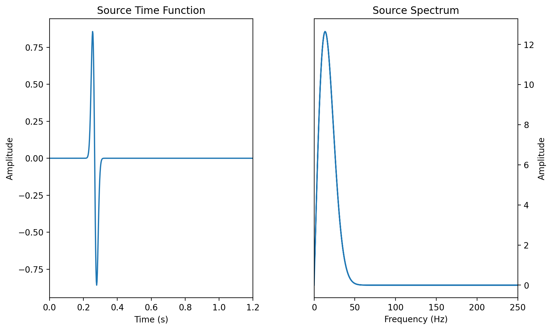
# Source time function (Gaussian)
# -------------------------------
src = np.zeros(nt + 1)
time = np.linspace(0 * dt, nt * dt, nt)
# 1st derivative of a Gaussian (corrected May 3, 2020)
src = -8.0 * (time - t0) * f0 * (np.exp(-1.0 * (4 * f0) ** 2 * (time - t0) ** 2))

# Plot source time function

# Plot position configuration
# ---------------------------
plt.ion()
fig1 = plt.figure(figsize=(10, 6))
gs1 = gridspec.GridSpec(1, 2, width_ratios=[1, 1], hspace=0.3, wspace=0.3)

# Plot source time function
# -------------------------
ax1 = plt.subplot(gs1[0])
ax1.plot(time, src)  # plot source time function
ax1.set_title("Source Time Function")
ax1.set_xlim(time[0], time[-1])
ax1.set_xlabel("Time (s)")
ax1.set_ylabel("Amplitude")

# Plot source spectrum
# --------------------
ax2 = plt.subplot(gs1[1])
spec = np.fft.fft(src)  # source time function in frequency domain
freq = np.fft.fftfreq(
    spec.size, d=dt
)  # time domain to frequency domain (corrected May 3, 2020)
ax2.plot(np.abs(freq), np.abs(spec))  # plot frequency and amplitude
ax2.set_xlim(0, 250)  # only display frequency from 0 to 250 Hz
ax2.set_title("Source Spectrum")
ax2.set_xlabel("Frequency (Hz)")
ax2.set_ylabel("Amplitude")

ax2.yaxis.tick_right()
ax2.yaxis.set_label_position("right");

# Plot Snapshot & Seismogram - Run this code after simulation
# ---------------------------------------------------------------------------

# Initialize empty pressure
# -------------------------
p = np.zeros(nx)  # p at time n (now)
pold = np.zeros(nx)  # p at time n-1 (past)
pnew = np.zeros(nx)  # p at time n+1 (present)
d2px = np.zeros(nx)  # 2nd space derivative of p

# Initialize model (assume homogeneous model)
# -------------------------------------------
c = np.zeros(nx)
c = c + c0  # initialize wave velocity in model

# Initialize coordinate
# ---------------------
x = np.arange(nx)
x = x * dx  # coordinate in x-direction

# Initialize empty seismogram
# ---------------------------
seis = np.zeros(nt)

# Analytical solution
# -------------------
G = time * 0.0
for it in range(nt):  # Calculate Green's function (Heaviside function)
    if (time[it] - np.abs(x[ir] - x[isrc]) / c0) >= 0:
        G[it] = 1.0 / (2 * c0)
Gc = np.convolve(G, src * dt)
Gc = Gc[0:nt]
lim = Gc.max()  # get limit value from the maximum amplitude


# Plot position configuration
# ---------------------------
plt.ion()
fig2 = plt.figure(figsize=(10, 6))
gs2 = gridspec.GridSpec(1, 2, width_ratios=[1, 1], hspace=0.3, wspace=0.3)

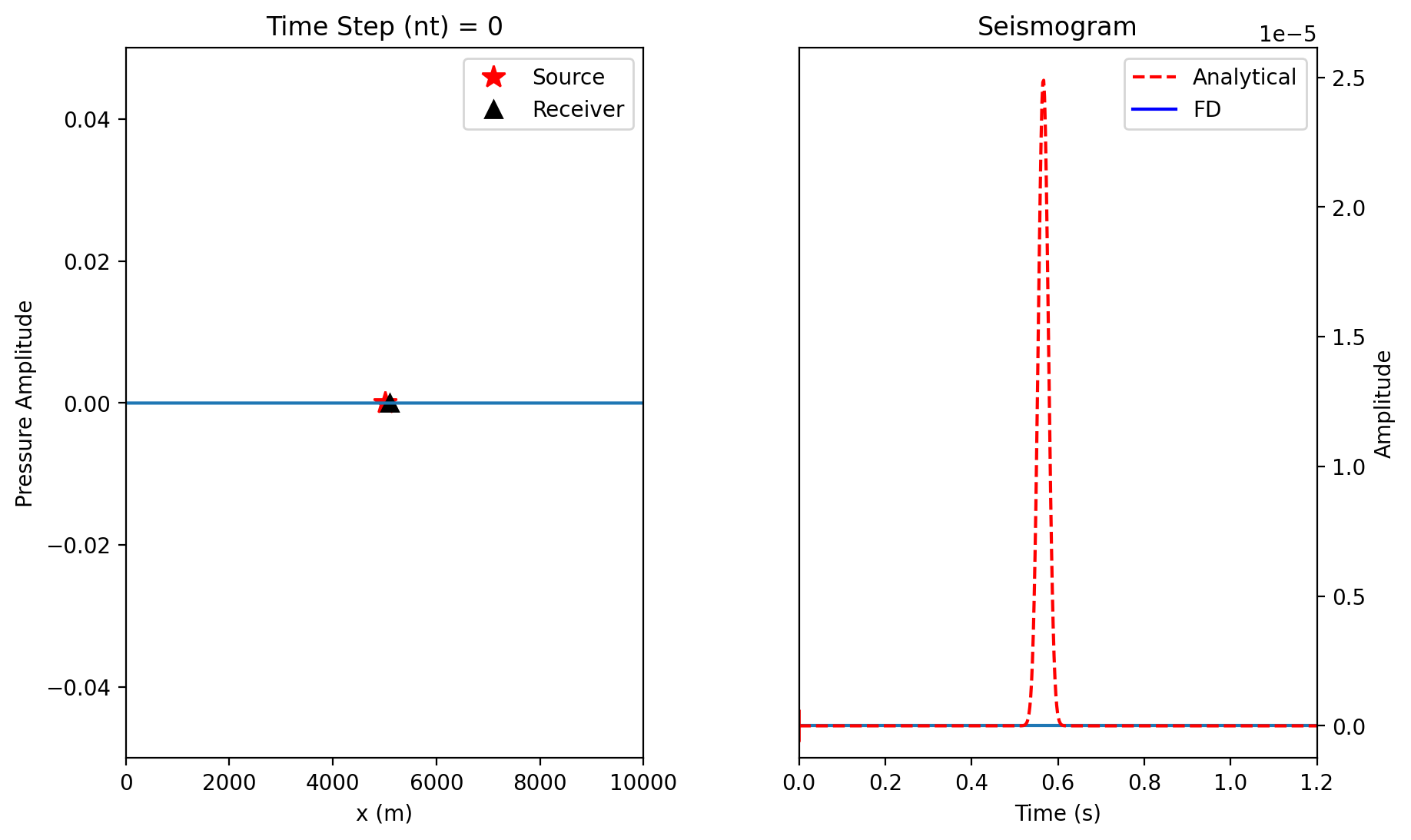
# Plot 1D wave propagation
# ------------------------
# Note: comma is needed to update the variable
ax3 = plt.subplot(gs2[0])
(leg1,) = ax3.plot(
    isrc, 0, "r*", markersize=11
)  # plot position of the source in snapshot
(leg2,) = ax3.plot(
    ir, 0, "k^", markersize=8
)  # plot position of the receiver in snapshot
(up31,) = ax3.plot(p)  # plot pressure update each time step
ax3.set_xlim(0, xmax)
ax3.set_ylim(-np.max(p), np.max(p))
ax3.set_title("Time Step (nt) = 0")
ax3.set_xlabel("x (m)")
ax3.set_ylabel("Pressure Amplitude")
ax3.legend(
    (leg1, leg2), ("Source", "Receiver"), loc="upper right", fontsize=10, numpoints=1
)

# Plot seismogram
# ---------------
# Note: comma is needed to update the variable
ax4 = plt.subplot(gs2[1])
(leg3,) = ax4.plot(0, 0, "r--", markersize=1)  # plot analytical solution marker
(leg4,) = ax4.plot(0, 0, "b-", markersize=1)  # plot numerical solution marker
(up41,) = ax4.plot(time, seis)  # update recorded seismogram each time step
(up42,) = ax4.plot([0], [0], "r|", markersize=15)  # update time step position
ax4.yaxis.tick_right()
ax4.yaxis.set_label_position("right")
ax4.set_xlim(time[0], time[-1])
ax4.set_title("Seismogram")
ax4.set_xlabel("Time (s)")
ax4.set_ylabel("Amplitude")
ax4.legend(
    (leg3, leg4), ("Analytical", "FD"), loc="upper right", fontsize=10, numpoints=1
)

plt.plot(time, Gc, "r--")  # plot analytical solution

[<matplotlib.lines.Line2D at 0x7f572ad3e150>]

# 1D Wave Propagation (Finite Difference Solution)
# ------------------------------------------------


# Calculate Partial Derivatives
# -----------------------------
for it in range(nt):
    if op == 3:  # use 3 point operator FD scheme
        for i in range(1, nx - 1):
            d2px[i] = (p[i + 1] - 2 * p[i] + p[i - 1]) / dx**2

    if op == 5:  # use 5 point operator FD scheme
        for i in range(2, nx - 2):
            d2px[i] = (
                -1.0 / 12 * p[i + 2]
                + 4.0 / 3 * p[i + 1]
                - 5.0 / 2 * p[i]
                + 4.0 / 3 * p[i - 1]
                - 1.0 / 12 * p[i - 2]
            ) / dx**2

    # Time Extrapolation
    # ------------------
    pnew = 2 * p - pold + c**2 * dt**2 * d2px

    # Add Source Term at isrc
    # -----------------------
    # Absolute pressure w.r.t analytical solution
    pnew[isrc] = pnew[isrc] + src[it] / (dx) * dt**2

    # Remap Time Levels
    # -----------------
    pold, p = p, pnew

    # Output Seismogram
    # -----------------
    seis[it] = p[ir]

    # Plot pressure field
    # -------------------------------------
    # Snapshot
    idisp = 5  # display frequency
    if (it % idisp) == 0:
        ax3.set_title("Time Step (nt) = %d" % it)
        ax3.set_ylim(np.min(p), 1.1 * np.max(p))
        # plot around propagating wave
        window = 100
        xshift = 25
        ax3.set_xlim(
            isrc * dx + c0 * it * dt - window * dx - xshift,
            isrc * dx + c0 * it * dt + window * dx - xshift,
        )
        up31.set_ydata(p)
        up41.set_ydata(seis)
        up42.set_data(time[it], seis[it])
        plt.gcf().canvas.draw()

---------------------------------------------------------------------------
RuntimeError                              Traceback (most recent call last)
Cell In[7], line 55
     53 up31.set_ydata(p)
     54 up41.set_ydata(seis)
---> 55 up42.set_data(time[it], seis[it])
     56 plt.gcf().canvas.draw()

File /usr/lib/python3.12/site-packages/matplotlib/lines.py:665, in Line2D.set_data(self, *args)
    662 else:
    663     x, y = args
--> 665 self.set_xdata(x)
    666 self.set_ydata(y)

File /usr/lib/python3.12/site-packages/matplotlib/lines.py:1289, in Line2D.set_xdata(self, x)
   1276 """
   1277 Set the data array for x.
   1278 
   (...)
   1286 set_ydata
   1287 """
   1288 if not np.iterable(x):
-> 1289     raise RuntimeError('x must be a sequence')
   1290 self._xorig = copy.copy(x)
   1291 self._invalidx = True

RuntimeError: x must be a sequence