14. DiffusionCrankNic.m

function [x, err] = TriDiagonal(a, b, c, f)
    % Solution of a linear system of equations with a tridiagonal
    % matrix.
    %
    %   a(k) x(k-1) + b(k) x(k) + c(k) x(k+1) = f(k)
    %
    % with a(1) = c(n) = 0.
    %
    % Input
    %   a(1:n), b(1:n), c(1:n) : the coefficients of the system
    %                            matrix
    %   f(1:n) : the right hand side vector
    %
    % Output
    %   x(1:n) : the solution to the linear system of equations, if
    %            no division by zero occurs
    %   err : = 0, if no division by zero occurs
    %         = 1, if division by zero is encountered
    n = length(f);
    alpha = zeros(n, 1);
    beta = zeros(n, 1);
    err = 0;

    if abs(b(1)) > eps(b(1))
        alpha(1) = -c(1) / b(1);
        beta(1) = f(1) / b(1);
    else
        err = 1;
        return;
    end

    for k = 2:n
        denominator = a(k) * alpha(k - 1) + b(k);

        if abs(denominator) > eps(denominator)
            alpha(k) =- c(k) / denominator;
            beta(k) = (f(k) - a(k) * beta(k - 1)) / denominator;
        else
            err = 1;
            return;
        end

    end

    if abs(a(n) * alpha(n - 1) + b(n)) > eps(b(n))
        x(n) = (f(n) - a(n) * beta(n - 1)) / (a(n) * alpha(n - 1) + b(n));
    else
        err = 1;
        return;
    end

    for k = n - 1:-1:1
        x(k) = alpha(k) * x(k + 1) + beta(k);
    end

end

warning: using the gnuplot graphics toolkit is discouraged

The gnuplot graphics toolkit is not actively maintained and has a number
of limitations that are unlikely to be fixed.  Communication with gnuplot
uses a one-directional pipe and limited information is passed back to the
Octave interpreter so most changes made interactively in the plot window
will not be reflected in the graphics properties managed by Octave.  For
example, if the plot window is closed with a mouse click, Octave will not
be notified and will not update its internal list of open figure windows.
The qt toolkit is recommended instead.

function frc = fForcing(N, t)
    %
    % Constructs the forcing term:
    %
    % Input
    %   N : to compute the mesh size
    %   t : the current time at the time interval midpoint
    %
    % Output
    %   f(1:N-1) : the array of values of the forcing function
    %
    frc = zeros(1, N - 1);
    h = 1.0 / N;

    for i = 1:N - 1
        x = i * h;
        tpx = 2.0 * pi * x;
        tpt = 2.0 * pi * t;
        frc(i) = 2.0 * pi * sin(tpt) * (1.0 - exp(sin(tpx))) ...
            + 4.0 * pi * pi * cos(tpt) * exp(sin(tpx)) ...
            * (sin(tpx) - cos(tpx) * cos(tpx));
    end

end

function ue = uExact(N, t)
    %
    % Constructs the exact solution:
    %
    % Input
    %   N : to compute the mesh size
    %   t : the current time
    %
    % Output
    %   ue(1:N+1) : the array of values of the exact solution
    %
    ue = zeros(1, N + 1);
    h = 1.0 / N;

    for i = 0:N
        x = i * h;
        tpx = 2.0 * pi * x;
        tpt = 2.0 * pi * t;
        ue(i + 1) = cos(tpt) * (exp(sin(tpx)) - 1.0);
    end

end

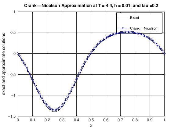
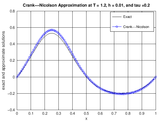
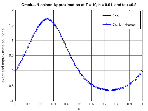
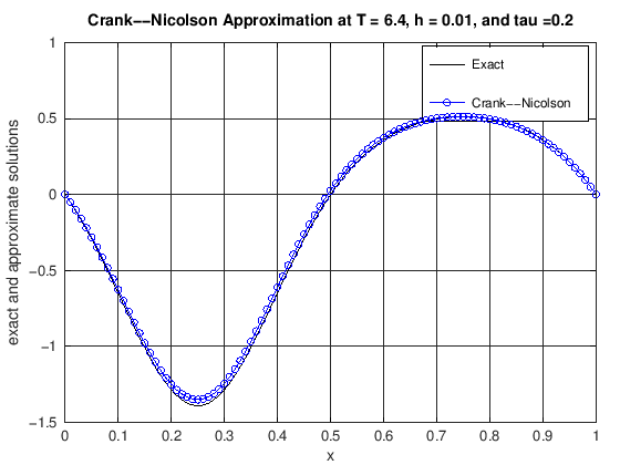
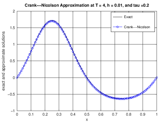
function [error] = DiffusionCrankNic(finalT, N, K, numPlots)
    %
    % This function computes numerical approximations to solutions
    % of the linear diffusion equation
    %
    % u_t - u_xx = f(x,t)
    %
    % using the Crank-Nicolson (CN) method on the domain [0,1]. The
    % forcing function, f, and the intial conditions are constructed
    % so that the true solution is
    %
    % u(x,t) = cos(2*pi*t)*(exp(sin(2*pi*x))-1.0).
    %
    % This can be easily modified.
    %
    % Input
    %   finalT : the final time
    %   N : the number of spatial grid points in [0,1]
    %   K : the number of time steps in the interval [0,finalT]
    %   numPlots : the number of output frames in the time interval
    %              [0,finalT]. numPlots must be a divisor of K.
    %
    % Output
    %   error: the max norm error of the CN scheme at t = finalT
    %
    error = 0.0;

    if N > 0 && N - floor(N) == 0
        h = 1.0 / N;
    else
        display('Error: N must be a positive integer.')
        return
    end

    if (K > 0 && K - floor(K) == 0) && finalT > 0
        tau = finalT / K;
    else
        display('Error: K must be a positive integer, and')
        display('       finalT must be positive.')
        return
    end

    mu = tau / (2.0 * h * h);

    x = 0:h:1.0;
    uoCN(1:N + 1) = uExact(N, 0.0);

    if mod(K, numPlots) == 0
        stepsPerPlot = K / numPlots;
    else
        display('Error: numPlots is not a divisor of K.')
        return
    end

    %
    % Define the tridiagonal system matrix to be inverted:
    %
    a(1) = 0.0;
    a(2:N - 1) = -mu;
    b(1:N - 1) = 1.0 + 2.0 * mu;
    c(1:N - 2) = -mu;
    c(N - 1) = 0.0;
    %
    % Main time loop:
    %
    for k = 1:numPlots

        for j = 1:stepsPerPlot
            kk = (k - 1) * stepsPerPlot + j;
            currTime = tau * (kk);
            lastTime = tau * (kk - 1.0);
            f(1:N - 1) = tau * (fForcing(N, currTime) ...
                +fForcing(N, lastTime)) / 2.0;

            for ell = 1:N - 1
                rhs(ell) = f(ell) + uoCN(ell + 1) + mu * (uoCN(ell) ...
                    -2.0 * uoCN(ell + 1) + uoCN(ell + 2));
            end

            [uCN(2:N), err] = TriDiagonal(a, b, c, rhs);
            uCN(1) = 0.0;
            uCN(N + 1) = 0.0;
            uoCN = uCN;
        end

        hf = figure(k);
        clf
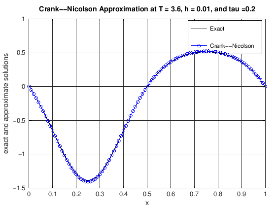
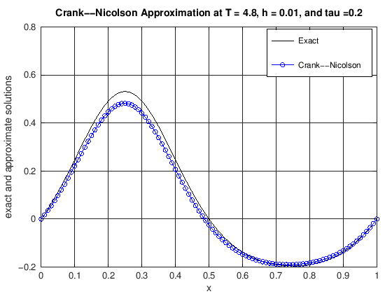
        plot(x, uExact(N, currTime), 'k-', x, uCN, 'b-o')
        grid on,
        xlabel("x");
        ylabel('exact and approximate solutions');
        title(['Crank--Nicolson Approximation at T = ', ...
                num2str(currTime), ', h = ', num2str(h), ...
                ', and tau =', num2str(tau)]);
        legend("Exact", "Crank--Nicolson")
        set(gca, "xTick", 0:0.1:1)

        s1 = ['000', num2str(k)];
        s2 = s1((length(s1) - 3):length(s1));
        s3 = ['OUT/diff', s2, '.pdf'];
        %exportgraphics(gca, s3)
    end

    error = max(abs(uExact(N, currTime) - uCN));
end

finalT = 10;
N = 100;
K = 50;
numPlots = 25;

[error] = DiffusionCrankNic(finalT, N, K, numPlots)

error = 0.019031