34. Acoustic Waves 2D - Homogeneous case#
This notebook covers the following aspects:
Implementation of the 2D acoustic wave equation
Understanding the input parameters for the simulation and the plots that are generated
Comparison with analytical solution
Note
Green’s function calculation corrected (May 2020)
Source term and spectrum calculation corrected (May 2020)
34.1. Stability (Courant criterion)#
The Courant criterion is defined as
With this information we can calculate the maximum possible and stable time step.
34.1.1. Analytical Solution#
In the code below we present the analytical solution for the acoustic wave equation
assuming constant velocity c and infinite space. Note that in 1D and 2D this equation is mathematically equivalent to the problem of SH wave propagation (i.e., shear waves polarised perpendicular to the plane through source and receiver). In 3D it is (only) descriptive of pressure (sound) waves.
Analytical solution for inhomogeneous partial differential equations (i.e., with non-zero source terms) are usually developed using the concept of Green’s functions \(G(x, t; x_0, t_0)\). Green’s functions are the solutions to the specific partial differential equations for \(\delta\)-function as source terms evaluated at \((x, t)\) and activated at \((x_0, t_0)\). Thus, we seek solutions to
where \(\Delta\) is the Laplace operator. We recall the definition of the \(\delta-\)function as a generalised function with
and
When comparing numerical with analytical solutions the functions that - in the limit - lead to the \(\delta-\)function will become very important. An example is the boxcar function
fulfilling these properties as \(dx\rightarrow0\). These functions are used to properly scale the source terms to obtain correct absolute amplitudes.
To describe analytical solutions for the acoustic wave equation we also make use of the unit step function, also known as the Heaviside function, defined as
The Heaviside function is the integral of the \(\delta-\)function (and vice-versa the \(\delta\)-function is defined as the derivative of the Heaviside function). In 2D case, the Green’s function is
A special situation occurs in 2D. An impulsive source leads to a waveform with a coda that decreases with time. This is a consequence of the fact that the source actually is a line source. From a computational point of view this is extremely important. Numerical solutions in 2D Cartesian coordinates cannot directly be compared to observations in which we usually have point sources.
34.1.2. Numerical Solution (Finite Differences Method)#
In 2D the constant-density acoustic wave equation is given by
where the \(z\)-coordinate is chosen because in many applications the \(x-z\) plane is considered a vertical plane with \(z\) as depth coordinate. In accordance with the above developments we discretise space-time using
Using the 3-point operator for the 2nd derivatives in time leads us to the extrapolation scheme
where on the r.h.s. the space and time dependencies are implicitly assumed and the partial derivatives are approximated by
\begin{equation} \begin{split} \partial_x^2 p \ &= \ \frac{p_{i+1,j}^{n} - 2 p_{i,j}^n + p_{i-1,j}^{n}}{dx^2} \ \partial_z^2 p \ &= \ \frac{p_{i,j+1}^{n} - 2 p_{i,j}^n + p_{i,j-1}^{n}}{dz^2} \ . \end{split} \end{equation} Note that for a regular 2D grid \(dz=dx\)
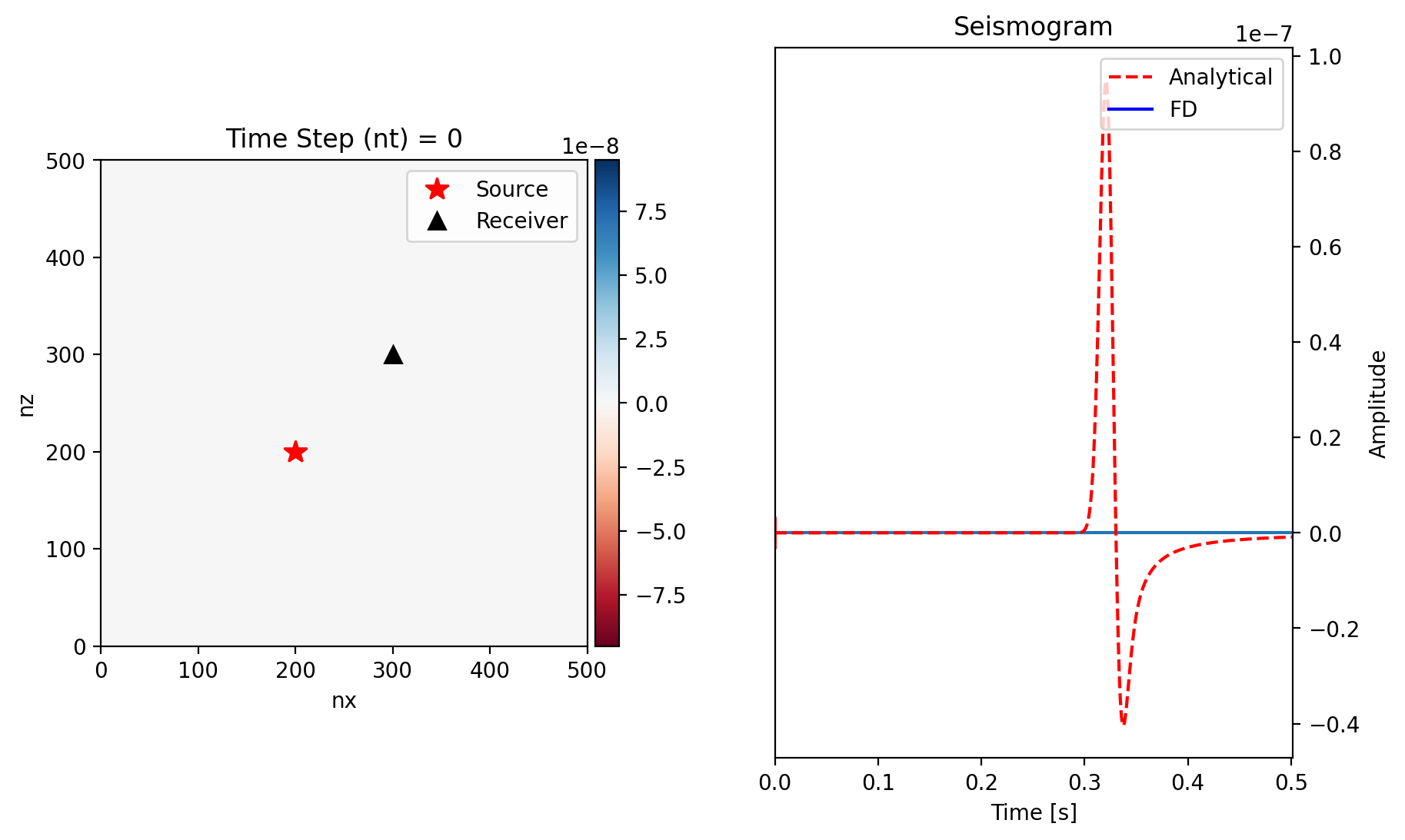
34.1.3. Analytical and Numerical Comparisons#
The code below is given with a 3-point difference operator. Compare the results from numerical simulation with the 3-point operator with the analytical solution.
34.1.4. High-order operators#
Extend the code by adding the option to use a 5-point difference operator. The 5-pt weights are: $\( [-1/12, 4/3, -5/2, 4/3, -1/12]/dx^2 \)$. Compare simulations with the 3-point and 5-point operators.
import warnings

import matplotlib
import matplotlib.pyplot as plt
import numpy as np
from matplotlib import gridspec, use
from mpl_toolkits.axes_grid1 import make_axes_locatable
# matplotlib.use("nbagg")
warnings.filterwarnings("ignore")
# Parameter Configuration
# -----------------------

nx = 500  # number of grid points in x-direction
nz = nx  # number of grid points in z-direction
# Note: regular 2D grid, dz = dx
dx = 1.0  # grid point distance in x-direction
dz = dx  # grid point distance in z-direction
c0 = 580.0  # wave velocity in medium (m/s)
isx = 200  # source location in grid in x-direction
isz = isx  # source location in grid in z-direction
irx = 300  # receiver location in grid in x-direction
irz = irx  # receiver location in grid in z-direction
nt = 502  # maximum number of time steps
dt = 0.0010  # time step
f0 = 25.0  # dominant frequency of the source (Hz)
t0 = 2.0 / f0  # source time shift
op = 3  # length of finite-difference operator (3 or 5)

print("Source frequency =", f0, "Hz")

# CFL Stability Criterion
# -----------------------
eps = c0 * dt / dx  # epsilon value
print("Stability criterion =", eps)

# Initialize Empty Pressure
# -------------------------
p = np.zeros((nz, nx))  # p at time n (now)
pold = np.zeros((nz, nx))  # p at time n-1 (past)
pnew = np.zeros((nz, nx))  # p at time n+1 (present)
d2px = np.zeros((nz, nx))  # 2nd space derivative of p in x-direction
d2pz = np.zeros((nz, nx))  # 2nd space derivative of p in z-direction

# Initialize Velocity Model (assume homogeneous model)
# ----------------------------------------------------
c = np.zeros((nz, nx))
c = c + c0  # initialize wave velocity in model

# Initialize Grid
x = np.arange(nx)
x = x * dx  # coordinate in x-direction
z = np.arange(nz)
z = z * dz  # coordinate in z-direction

# Initialize Empty Seismogram
# ---------------------------
seis = np.zeros(nt)

# Fontsize
# fs=20
Source frequency = 25.0 Hz
Stability criterion = 0.58
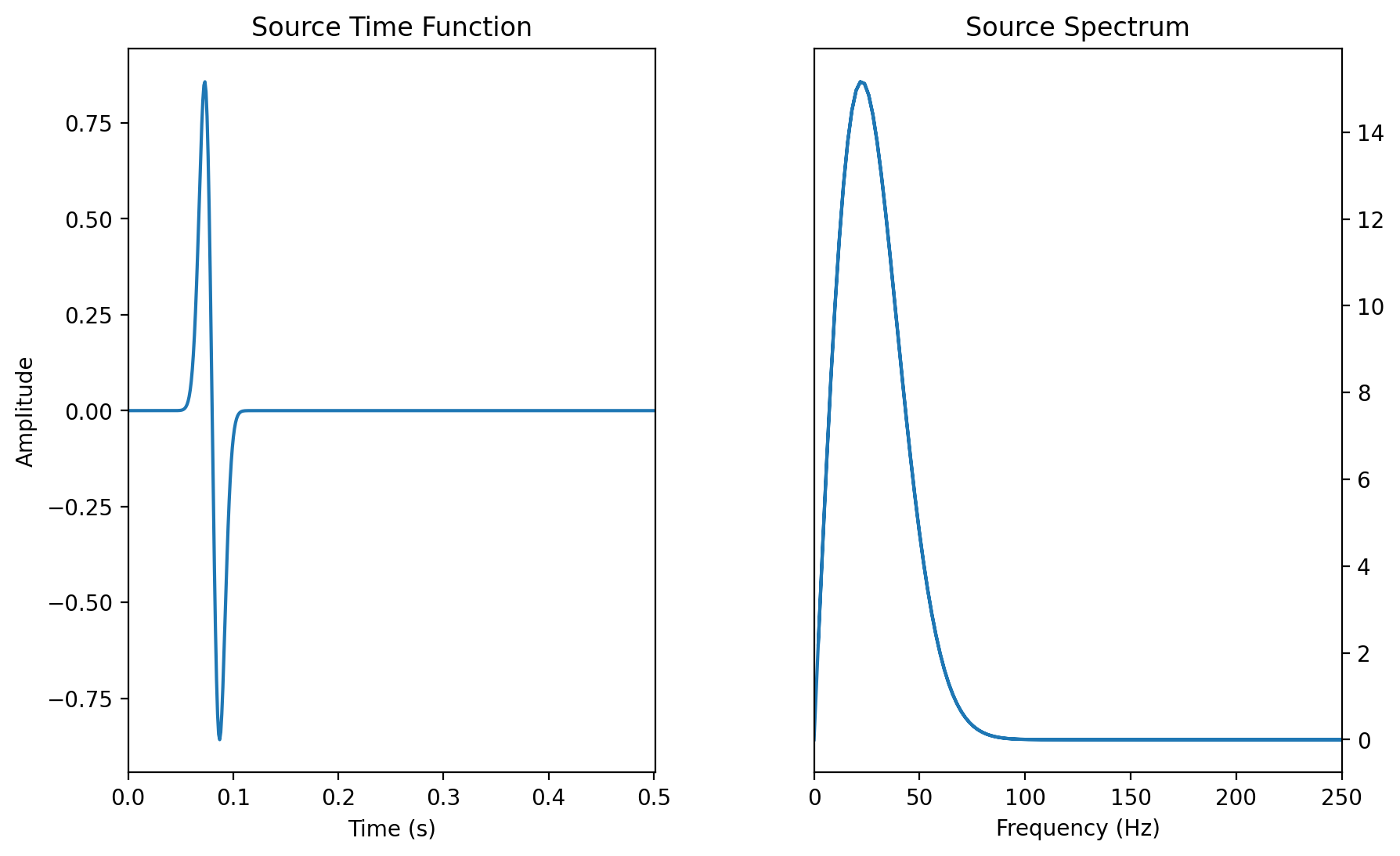
# Initialize Source Time Function
# -------------------------
# Source time function (Gaussian)
# -------------------------------
src = np.zeros(nt + 1)
time = np.linspace(0 * dt, nt * dt, nt)
# 1st derivative of a Gaussian
src = -8.0 * (time - t0) * f0 * (np.exp(-1.0 * (4 * f0) ** 2 * (time - t0) ** 2))
# Plot Source Time Function
# -------------------------

# Plot Position Configuration
# ---------------------------
plt.ion()
fig1 = plt.figure(figsize=(10, 6))
gs1 = gridspec.GridSpec(1, 2, width_ratios=[1, 1], hspace=0.3, wspace=0.3)

# Plot Source Time Function
# -------------------------
ax1 = plt.subplot(gs1[0])
ax1.plot(time, src)  # plot source time function
ax1.set_title("Source Time Function")
ax1.set_xlim(time[0], time[-1])
ax1.set_xlabel("Time (s)")
ax1.set_ylabel("Amplitude")

# Plot Source Spectrum
# --------------------
ax2 = plt.subplot(gs1[1])
spec = np.fft.fft(src)  # source time function in frequency domain
freq = np.fft.fftfreq(spec.size, d=dt)  # time domain to frequency domain
ax2.plot(np.abs(freq), np.abs(spec))  # plot frequency and amplitude
ax2.set_xlim(0, 250)  # only display frequency from 0 to 250 Hz
ax2.set_title("Source Spectrum")
ax2.set_xlabel("Frequency (Hz)")

ax2.yaxis.tick_right()
ax2.yaxis.set_label_position("right")

plt.show()
# Plot Snapshot & Seismogram (PLEASE RERUN THIS CODE AGAIN AFTER SIMULATION!)
# ---------------------------------------------------------------------------

# Analytical Solution
# -------------------
G = time * 0.0
r = np.sqrt((x[isx] - x[irx]) ** 2 + (z[isz] - z[irz]) ** 2)

for it in range(nt):  # Calculate Green's function
    # if ((time[it] - np.abs(x[irx] - x[isx]) / c0) >= 0):
    if (time[it] - r / c0) >= 0:
        G[it] = (1.0 / (2 * np.pi * c0**2)) * (
            1.0 / np.sqrt((time[it] ** 2) - (r**2 / (c0**2)))
        )
Gc = np.convolve(G, src * dt)
Gc = Gc[0:nt]
lim = Gc.max()  # get limit value from maximum amplitude of analytical solution

# Plot Position Configuration
# ---------------------------
plt.ion()
fig2 = plt.figure(figsize=(10, 6))
gs2 = gridspec.GridSpec(1, 2, width_ratios=[1, 1], hspace=0.3, wspace=0.3)

# Plot 2D Wave Propagation
# ------------------------
# Note: comma is needed to update the variable
ax3 = plt.subplot(gs2[0])
(leg1,) = ax3.plot(
    isx, isz, "r*", markersize=11
)  # plot position of the source in model
(leg2,) = ax3.plot(
    irx, irz, "k^", markersize=8
)  # plot position of the receiver in model
im3 = ax3.imshow(p, vmin=-lim, vmax=+lim, interpolation="nearest", cmap=plt.cm.RdBu)
div = make_axes_locatable(ax3)
cax = div.append_axes("right", size="5%", pad=0.05)  # size & position of colorbar
fig2.colorbar(im3, cax=cax)  # plot colorbar
ax3.set_title("Time Step (nt) = 0")
ax3.set_xlim(0, nx)
ax3.set_ylim(0, nz)
ax3.set_xlabel("nx")
ax3.set_ylabel("nz")
ax3.legend(
    (leg1, leg2), ("Source", "Receiver"), loc="upper right", fontsize=10, numpoints=1
)

# Plot Seismogram
# ---------------
# Note: comma is needed to update the variable
ax4 = plt.subplot(gs2[1])
(up41,) = ax4.plot(time, seis)  # update seismogram each time step
(up42,) = ax4.plot([0], [0], "r|", markersize=15)  # update time step position
ax4.set_xlim(time[0], time[-1])
ax4.set_title("Seismogram")
ax4.set_xlabel("Time [s]")
ax4.set_ylabel("Amplitude")
(leg3,) = ax4.plot(0, 0, "r--", markersize=1)
(leg4,) = ax4.plot(0, 0, "b-", markersize=1)
ax4.legend(
    (leg3, leg4), ("Analytical", "FD"), loc="upper right", fontsize=10, numpoints=1
)

ax4.yaxis.tick_right()
ax4.yaxis.set_label_position("right")

plt.plot(time, Gc, "r--")
plt.show()
# 2D Wave Propagation (Finite Difference Solution)
# ------------------------------------------------


# Calculate Partial Derivatives
# -----------------------------
for it in range(nt):
    if op == 3:  # use 3 point operator FD scheme
        for i in range(1, nx - 1):
            d2px[i, :] = (p[i - 1, :] - 2 * p[i, :] + p[i + 1, :]) / dx**2
        for j in range(1, nz - 1):
            d2pz[:, j] = (p[:, j - 1] - 2 * p[:, j] + p[:, j + 1]) / dz**2

    if op == 5:  # use 5 point operator FD scheme
        # -----------------------------------------------#
        #     IMPLEMENT 5 POINT OPERATOR CODE HERE!     #
        # -----------------------------------------------#
        pass

    # Time Extrapolation
    # ------------------
    pnew = 2 * p - pold + (c**2) * (dt**2) * (d2pz + d2px)

    # Add Source Term at isz and isx
    # ------------------------------
    # Absolute pressure w.r.t analytical solution
    pnew[isz, isx] = pnew[isz, isx] + src[it] / (dx * dz) * (dt**2)

    # Remap Time Levels
    # -----------------
    pold, p = p, pnew

    # Output Seismogram
    # -----------------
    seis[it] = p[irz, irx]

    # Update Data for Wave Propagation Plot
    # -------------------------------------
    idisp = 5  # display frequency
    if (it % idisp) == 0:
        ax3.set_title("Time Step (nt) = %d" % it)
        ax3.imshow(p, vmin=-lim, vmax=+lim, interpolation="nearest", cmap=plt.cm.RdBu)
        up41.set_ydata(seis)
        up42.set_data(time[it], seis[it])
        # Uncoment for bigger fontsize - also uncoment the Fontsize in the cell parameters
        # for item in ([ax3.title, ax3.xaxis.label, ax3.yaxis.label] +
        #     ax3.get_xticklabels() + ax3.get_yticklabels()):
        #     item.set_fontsize(fs)
        # for item in ([ax4.title, ax4.xaxis.label, ax4.yaxis.label] +
        #     ax4.get_xticklabels() + ax4.get_yticklabels()):
        #     item.set_fontsize(fs)
        plt.gcf().canvas.draw()
---------------------------------------------------------------------------
RuntimeError                              Traceback (most recent call last)
Cell In[7], line 44
     42 ax3.imshow(p, vmin=-lim, vmax=+lim, interpolation="nearest", cmap=plt.cm.RdBu)
     43 up41.set_ydata(seis)
---> 44 up42.set_data(time[it], seis[it])
     45 # Uncoment for bigger fontsize - also uncoment the Fontsize in the cell parameters
     46 # for item in ([ax3.title, ax3.xaxis.label, ax3.yaxis.label] +
     47 #     ax3.get_xticklabels() + ax3.get_yticklabels()):
   (...)
     50 #     ax4.get_xticklabels() + ax4.get_yticklabels()):
     51 #     item.set_fontsize(fs)
     52 plt.gcf().canvas.draw()

File /usr/lib/python3.12/site-packages/matplotlib/lines.py:665, in Line2D.set_data(self, *args)
    662 else:
    663     x, y = args
--> 665 self.set_xdata(x)
    666 self.set_ydata(y)

File /usr/lib/python3.12/site-packages/matplotlib/lines.py:1289, in Line2D.set_xdata(self, x)
   1276 """
   1277 Set the data array for x.
   1278
   (...)
   1286 set_ydata
   1287 """
   1288 if not np.iterable(x):
-> 1289     raise RuntimeError('x must be a sequence')
   1290 self._xorig = copy.copy(x)
   1291 self._invalidx = True

RuntimeError: x must be a sequence