2. Finite-Difference Approximations

import matplotlib.pyplot as plt
import numpy as np
from helper import Approx, cleaner
from jaxtyping import Array, Float
from sympy import Derivative as D
from sympy import (
    Eq,
    Function,
    Matrix,
    O,
    Symbol,
    Wild,
    cos,
    solve,
    solve_linear_system,
    symbols,
)
from tabulate import tabulate

x = symbols("x")
h = symbols("h", positive=True)
f = Function("f")

2.1. They Taylor Series

2.1.1. Forward Taylor Series

Eq(f(x + h), f(x + h).series(x=h, x0=0, n=5).simplify())

\[\displaystyle f{\left(h + x \right)} = f{\left(x \right)} + h \frac{d}{d x} f{\left(x \right)} + \frac{h^{2} \frac{d^{2}}{d x^{2}} f{\left(x \right)}}{2} + \frac{h^{3} \frac{d^{3}}{d x^{3}} f{\left(x \right)}}{6} + \frac{h^{4} \frac{d^{4}}{d x^{4}} f{\left(x \right)}}{24} + O\left(h^{5}\right)\]

2.1.2. Backward Taylor Series

Eq(f(x - h), f(x - h).series(x=h, x0=0, n=5).simplify())

\[\displaystyle f{\left(- h + x \right)} = f{\left(x \right)} - h \frac{d}{d x} f{\left(x \right)} + \frac{h^{2} \frac{d^{2}}{d x^{2}} f{\left(x \right)}}{2} - \frac{h^{3} \frac{d^{3}}{d x^{3}} f{\left(x \right)}}{6} + \frac{h^{4} \frac{d^{4}}{d x^{4}} f{\left(x \right)}}{24} + O\left(h^{5}\right)\]

2.1.3. Truncating the Taylor series

2.1.4. Truncation error

Approx(cos(x + h), cos(x + h).series(x=h, x0=0, n=2).removeO().simplify())

\[\displaystyle \cos{\left(h + x \right)} \approx - h \sin{\left(x \right)} + \cos{\left(x \right)}\]

x = 0
h = 0.1
exact = np.cos(x + h)
first_order_approximation = np.cos(x) - h * np.sin(x)
truncation_error = np.abs(exact - first_order_approximation)
E_h = np.abs(-(np.power(h, 2)) / 2 * np.cos(x))

print(
    f"Truncation error: {truncation_error}\nE({h}): {E_h}\nError: {np.abs(truncation_error - E_h)}"
)

Truncation error: 0.0049958347219741794
E(0.1): 0.005000000000000001
Error: 4.165278025821534e-06

2.1.5. Plot

h = np.flip(np.reciprocal(2 ** np.arange(1, 5).astype(float)))
x = 1

h

array([0.0625, 0.125 , 0.25  , 0.5   ])

error_truncation = np.abs(np.cos(x + h) - (np.cos(x) - h * np.sin(x)))

error_truncation

array([0.0010207 , 0.00394192, 0.0146122 , 0.04882961])

h_values = np.linspace(start=0, stop=h.max())
E_h = np.abs(-1 / 2 * h_values**2 * np.cos(x))

fig, ax = plt.subplots()
ax.plot(
    h,
    error_truncation,
    "bo-",
    label=r"Truncation error: $|\cos(x+h) - (\cos(x) - h\sin(x))|$",
)
ax.plot(h_values, E_h, "r--", label=r"$E(h)=|-\frac{1}{2}h^2\cos(1)|$")
ax.set_xlabel("$h$")
ax.set_ylabel("Truncation error")
ax.set_title("Truncation error plot")
ax.grid()
legend = ax.legend(loc="best", shadow=True)

2.2. Big-oh notation

2.2.1. Expresing the truncation error as \(O\left(h^{n+1}\right)\)

2.2.2. Properties of \(O\left(h^{n}\right)\)

h = symbols("h")
m, n, k = (5, 2, -2)
assert m > n
k * O(h**n) == O(h**n)

True

O(h**m) + O(h**n) == O(h**n)

True

m, n = (2, 5)
assert m < n
O(h**n) / h**m == O(h ** (n - m))

True

2.3. Deriving finite-difference approximations

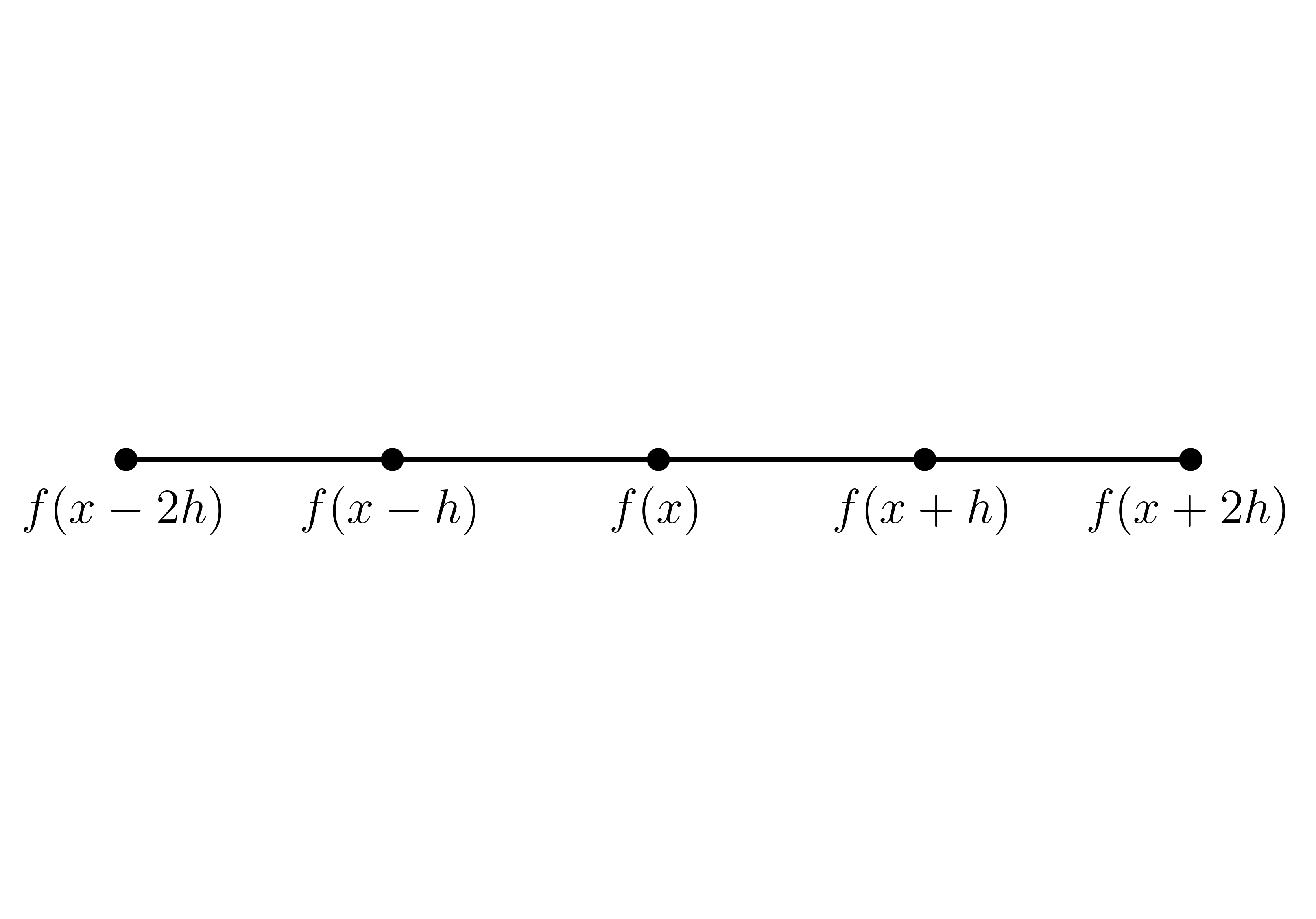
x = np.arange(-2, 3)

fig, ax = plt.subplots()
ax.plot(x, np.zeros_like(x), "ko-")
ax.text(x[0], -0.008, rf"$f(x-2h)$", ha="center", fontsize=15)
ax.text(x[1], -0.008, rf"$f(x-h)$", ha="center", fontsize=15)
ax.text(x[2], -0.008, rf"$f(x)$", ha="center", fontsize=15)
ax.text(x[3], -0.008, rf"$f(x+h)$", ha="center", fontsize=15)
ax.text(x[-1], -0.008, rf"$f(x+2h)$", ha="center", fontsize=15)
ax.axes.get_xaxis().set_visible(False)
ax.axes.get_yaxis().set_visible(False)
ax.set_frame_on(False)

2.3.1. First-order accurate finite difference approximation of \(f_{x}\left(x\right)\)

x = symbols("x")
h = symbols("h", positive=True)
f = Function("f")

Eq(f(x + h), f(x + h).series(x=h, x0=0, n=2).simplify())

\[\displaystyle f{\left(h + x \right)} = f{\left(x \right)} + h \frac{d}{d x} f{\left(x \right)} + O\left(h^{2}\right)\]

Eq(D(f(x)), solve(Eq(f(x + h), f(x + h).series(x=h, x0=0, n=2).simplify()), D(f(x)))[0])

\[\displaystyle \frac{d}{d x} f{\left(x \right)} = \frac{f{\left(h + x \right)} - f{\left(x \right)} + O\left(h^{2}\right)}{h}\]

2.3.2. First-order forward difference

_ = f(x + h).series(x=h, x0=0, n=2).removeO().simplify()
forward_difference = Approx(D(f(x)), solve(Eq(_, f(x + h)), D(f(x)))[0])

forward_difference

\[\displaystyle \frac{d}{d x} f{\left(x \right)} \approx \frac{- f{\left(x \right)} + f{\left(h + x \right)}}{h}\]

Eq(f(x - h), f(x - h).series(x=h, x0=0, n=2).simplify())

\[\displaystyle f{\left(- h + x \right)} = f{\left(x \right)} - h \frac{d}{d x} f{\left(x \right)} + O\left(h^{2}\right)\]

Eq(D(f(x)), solve(Eq(f(x - h), f(x - h).series(x=h, x0=0, n=2).simplify()), D(f(x)))[0])

\[\displaystyle \frac{d}{d x} f{\left(x \right)} = \frac{- f{\left(- h + x \right)} + f{\left(x \right)} + O\left(h^{2}\right)}{h}\]

2.3.3. First-order backward difference

_ = f(x - h).series(x=h, x0=0, n=2).removeO().simplify()
backward_difference = Approx(D(f(x)), solve(Eq(_, f(x - h)), D(f(x)))[0])

backward_difference

\[\displaystyle \frac{d}{d x} f{\left(x \right)} \approx \frac{f{\left(x \right)} - f{\left(- h + x \right)}}{h}\]

2.3.4. Second-order accurate finite difference approximation of \(f_{x}\left(x\right)\)

Eq(f(x + h), f(x + h).series(x=h, x0=0, n=3).simplify())

\[\displaystyle f{\left(h + x \right)} = f{\left(x \right)} + h \frac{d}{d x} f{\left(x \right)} + \frac{h^{2} \frac{d^{2}}{d x^{2}} f{\left(x \right)}}{2} + O\left(h^{3}\right)\]

Eq(f(x - h), f(x - h).series(x=h, x0=0, n=3).simplify())

\[\displaystyle f{\left(- h + x \right)} = f{\left(x \right)} - h \frac{d}{d x} f{\left(x \right)} + \frac{h^{2} \frac{d^{2}}{d x^{2}} f{\left(x \right)}}{2} + O\left(h^{3}\right)\]

Eq(
    f(x + h) - f(x - h),
    f(x + h).series(x=h, x0=0, n=3).simplify()
    - f(x - h).series(x=h, x0=0, n=3).simplify(),
)

\[\displaystyle - f{\left(- h + x \right)} + f{\left(h + x \right)} = 2 h \frac{d}{d x} f{\left(x \right)} + O\left(h^{3}\right)\]

2.3.5. Second-order central difference

_ = f(x + h).series(x=h, x0=0, n=3).removeO().simplify()
__ = f(x - h).series(x=h, x0=0, n=3).removeO().simplify()
central_difference = Approx(
    D(f(x), x), solve(Eq(_ - __, f(x + h) - f(x - h)), D(f(x), x))[0]
)

central_difference

\[\displaystyle \frac{d}{d x} f{\left(x \right)} \approx \frac{- f{\left(- h + x \right)} + f{\left(h + x \right)}}{2 h}\]

2.3.6. Second-order accurate finite difference approximation of \(f_{xx}\left(x\right)\)

Eq(f(x + h), f(x + h).series(x=h, x0=0, n=4).simplify())

\[\displaystyle f{\left(h + x \right)} = f{\left(x \right)} + h \frac{d}{d x} f{\left(x \right)} + \frac{h^{2} \frac{d^{2}}{d x^{2}} f{\left(x \right)}}{2} + \frac{h^{3} \frac{d^{3}}{d x^{3}} f{\left(x \right)}}{6} + O\left(h^{4}\right)\]

Eq(f(x - h), f(x - h).series(x=h, x0=0, n=4).simplify())

\[\displaystyle f{\left(- h + x \right)} = f{\left(x \right)} - h \frac{d}{d x} f{\left(x \right)} + \frac{h^{2} \frac{d^{2}}{d x^{2}} f{\left(x \right)}}{2} - \frac{h^{3} \frac{d^{3}}{d x^{3}} f{\left(x \right)}}{6} + O\left(h^{4}\right)\]

Eq(
    f(x + h) + f(x - h),
    f(x + h).series(x=h, x0=0, n=4).simplify()
    + f(x - h).series(x=h, x0=0, n=4).simplify(),
)

\[\displaystyle f{\left(- h + x \right)} + f{\left(h + x \right)} = 2 f{\left(x \right)} + h^{2} \frac{d^{2}}{d x^{2}} f{\left(x \right)} + O\left(h^{4}\right)\]

2.3.7. Second-order symmetric difference

_ = f(x + h).series(x=h, x0=0, n=4).removeO().simplify()
__ = f(x - h).series(x=h, x0=0, n=4).removeO().simplify()
symmetric_difference = Approx(
    D(f(x), x, 2), solve(Eq(_ + __, f(x + h) + f(x - h)), D(f(x), x, 2))[0]
)

symmetric_difference

\[\displaystyle \frac{d^{2}}{d x^{2}} f{\left(x \right)} \approx \frac{- 2 f{\left(x \right)} + f{\left(- h + x \right)} + f{\left(h + x \right)}}{h^{2}}\]

cleaner(["x", "h", "f"])

Symbolic variables already cleared

2.3.8. Example \(3\)

def forward_first_derivative(
    f: np.ufunc, x: float, h: Float[Array, "dim1"]
) -> Float[Array, "dim1"]:
    return (f(x + h) - f(x)) / h


def backward_first_derivative(
    f: np.ufunc, x: float, h: Float[Array, "dim1"]
) -> Float[Array, "dim1"]:
    return (f(x) - f(x - h)) / h


def central_first_derivative(
    f: np.ufunc, x: float, h: Float[Array, "dim1"]
) -> Float[Array, "dim1"]:
    return (f(x + h) - f(x - h)) / (2 * h)


def central_second_derivative(
    f: np.ufunc, x: float, h: Float[Array, "dim1"]
) -> Float[Array, "dim1"]:
    return (f(x + h) - 2 * f(x) + f(x - h)) / h**2

f = np.cos
f_prime = lambda x: -np.sin(x)
f_prime_prime = lambda x: -np.cos(x)
x = np.pi / 4
h = np.array(0.1)
exact_first_derivative = f_prime(x)
exact_second_derivative = f_prime_prime(x)

ffd = forward_first_derivative(f=f, x=x, h=h)
bfd = backward_first_derivative(f=f, x=x, h=h)
cfd = central_first_derivative(f=f, x=x, h=h)
csd = central_second_derivative(f=f, x=x, h=h)

print(
    f"First derivative: {exact_first_derivative}\nForward first derivative: {ffd}\nBackward first derivative: {bfd}\
\nCentral first derivative: {cfd}\nSecond derivative: {exact_second_derivative}\nCentral second derivative: {csd}"
)

First derivative: -0.7071067811865475
Forward first derivative: -0.741254745095894
Backward first derivative: -0.6706029729039886
Central first derivative: -0.7059288589999413
Second derivative: -0.7071067811865476
Central second derivative: -0.7065177219190532

error_ffd = np.abs(exact_first_derivative - ffd)
error_bfd = np.abs(exact_first_derivative - bfd)
error_cfd = np.abs(exact_first_derivative - cfd)
error_csd = np.abs(exact_second_derivative - csd)

print(
    f"Error forward first derivative: {error_ffd}\nError backward first derivative: {error_bfd}\
\nError central first derivative: {error_cfd}\nError central second derivative: {error_csd}"
)

Error forward first derivative: 0.03414796390934649
Error backward first derivative: 0.036503808282558836
Error central first derivative: 0.0011779221866061729
Error central second derivative: 0.0005890592674944184

2.3.9. Estimating the order of an approximation

\[ n\approx \dfrac{\log\left|E\left(h_{\max}\right)\right| -\log\left|E\left(h_{\min}\right)\right|}{ \log\left(h_{\max}\right)-\log\left(h_{\min}\right) }. \]

def estimate_order(
    h: Float[Array, "dim1"], truncation_error: Float[Array, "dim1"]
) -> float:
    assert h.size == truncation_error.size

    Eh_max = truncation_error[np.argmax(h, axis=0)[0]][0]
    Eh_min = truncation_error[np.argmin(h, axis=0)[0]][0]

    return (np.log(np.abs(Eh_max)) - np.log(np.abs(Eh_min))) / (
        np.log(h.max()) - np.log(h.min())
    )

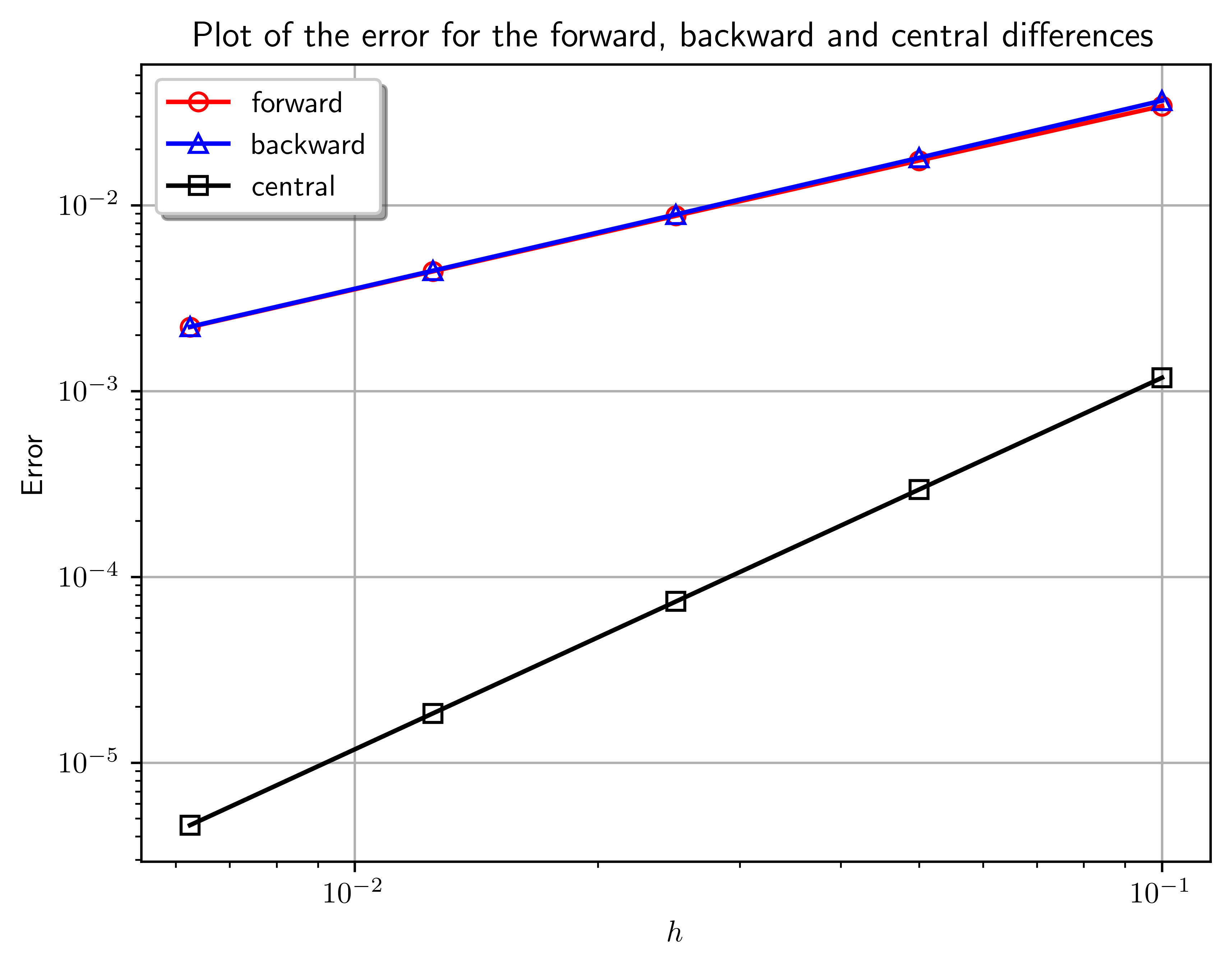
2.3.10. Table 2.1

Finite-difference approximations of the first derivative of \(f\left(x\right)=\cos\left(x\right)\) at \(x=\dfrac{\pi}{4}\) using step lengths \(h\in\left\{0.1,0.05,0.25,0.0125,0.00625\right\}\).

f = np.cos
f_prime = lambda x: -np.sin(x)
x = np.pi / 4
h = np.reciprocal(10 * (2 ** np.arange(5).astype(float)))[np.newaxis].T

h

array([[0.1    ],
       [0.05   ],
       [0.025  ],
       [0.0125 ],
       [0.00625]])

forward = forward_first_derivative(f=f, x=x, h=h)
backward = backward_first_derivative(f=f, x=x, h=h)
central = central_first_derivative(f=f, x=x, h=h)

tabular = np.concatenate((h, forward, backward, central), axis=1)
header = ["h", "Forward", "Backward", "Central"]

print(
    tabulate(tabular_data=tabular, headers=header, floatfmt=(".5e"))
)  # TODO: As xarray.

          h       Forward      Backward       Central
-----------  ------------  ------------  ------------
1.00000e-01  -7.41255e-01  -6.70603e-01  -7.05929e-01
5.00000e-02  -7.24486e-01  -6.89138e-01  -7.06812e-01
2.50000e-02  -7.15872e-01  -6.98195e-01  -7.07033e-01
1.25000e-02  -7.11508e-01  -7.02669e-01  -7.07088e-01
6.25000e-03  -7.09312e-01  -7.04892e-01  -7.07102e-01

print(f"{f_prime(x):.5e}")

-7.07107e-01

error_forward = np.abs(f_prime(x) - forward)
error_backward = np.abs(f_prime(x) - backward)
error_central = np.abs(f_prime(x) - central)

fig, ax = plt.subplots()
ax.loglog(h, error_forward, "ro-", mfc="none", label="forward")
ax.loglog(h, error_backward, "b^-", mfc="none", label="backward")
ax.loglog(h, error_central, "ks-", mfc="none", label="central")
ax.set_xlabel(r"$h$")
ax.set_ylabel(r"Error")
ax.set_title("Plot of the error for the forward, backward and central differences")
ax.grid()
legend = ax.legend(loc="best", shadow=True)

2.3.11. Table 2.2

Truncation errors for the Taylor series approximations of \(\cos\left(1+h\right)\) for \(h\in\left\{0.5,0.25,0.125,0.0625\right\}\).

f = lambda h: np.cos(1 + h)
f_prime = lambda h: -np.sin(1 + h)
x = 1
h = np.reciprocal(2 ** np.arange(1, 5).astype(float))[np.newaxis].T

h

array([[0.5   ],
       [0.25  ],
       [0.125 ],
       [0.0625]])

forward = forward_first_derivative(f=f, x=x, h=h)
backward = backward_first_derivative(f=f, x=x, h=h)
central = central_first_derivative(f=f, x=x, h=h)

error_forward = np.abs(f_prime(x) - forward)
error_backward = np.abs(f_prime(x) - backward)
error_central = np.abs(f_prime(x) - central)

tabular = np.concatenate((h, error_forward, error_backward, error_central), axis=1)
header = ["h", "Forward error", "Backward error", "Central error"]

print(tabulate(tabular_data=tabular, headers=header, floatfmt=(".5e")))

          h    Forward error    Backward error    Central error
-----------  ---------------  ----------------  ---------------
5.00000e-01      1.39304e-01       6.44706e-02      3.74166e-02
2.50000e-01      6.11903e-02       4.23057e-02      9.44229e-03
1.25000e-01      2.83414e-02       2.36092e-02      2.36611e-03
6.25000e-02      1.35922e-02       1.24085e-02      5.91875e-04

estimate_order(h, error_forward)

np.float64(1.1191270541574243)

estimate_order(h, error_backward)

np.float64(0.7924386666069776)

estimate_order(h, error_central)

np.float64(1.9940809174948577)

2.3.12. Finite-difference approximations of mixed derivatives

x, y = symbols("x y")
dx = Symbol(r"\Delta x")
dy = Symbol(r"\Delta y")
f = Function("f")
arg1, arg2 = Wild("arg1"), Wild("arg2")

_ = Approx(f(x + dx, y), f(x + dx, y).series(x=dx, x0=0, n=2).removeO().simplify())

__ = Approx(f(x, y + dy), f(x, y + dy).series(x=dy, x0=0, n=2).removeO().simplify())

Eq1 = Approx(D(f(x, y), x), solve(_, D(f(x, y), x))[0])

Eq2 = Approx(D(f(x, y), y), solve(__, D(f(x, y), y))[0])

Eq1

\[\displaystyle \frac{\partial}{\partial x} f{\left(x,y \right)} \approx \frac{- f{\left(x,y \right)} + f{\left(\Delta x + x,y \right)}}{\Delta x}\]

Eq2

\[\displaystyle \frac{\partial}{\partial y} f{\left(x,y \right)} \approx \frac{- f{\left(x,y \right)} + f{\left(x,\Delta y + y \right)}}{\Delta y}\]

Approx(
    D(D(f(x, y), y), x),
    Eq1.rhs.replace(f(arg1, arg2), D(f(arg1, arg2), arg2)),
)

\[\displaystyle \frac{\partial^{2}}{\partial x\partial y} f{\left(x,y \right)} \approx \frac{- \frac{\partial}{\partial y} f{\left(x,y \right)} + \frac{\partial}{\partial y} f{\left(\Delta x + x,y \right)}}{\Delta x}\]

Approx(
    D(D(f(x, y), y), x),
    Eq1.rhs.replace(f(arg1, arg2), D(f(arg1, arg2), arg2)).subs(
        {
            D(f(x + dx, y), y): Eq2.rhs.replace(f(arg1, arg2), f(arg1 + dx, arg2)),
            D(f(x, y), y): Eq2.rhs,
        }
    ),
)

\[\displaystyle \frac{\partial^{2}}{\partial x\partial y} f{\left(x,y \right)} \approx \frac{- \frac{- f{\left(x,y \right)} + f{\left(x,\Delta y + y \right)}}{\Delta y} + \frac{- f{\left(\Delta x + x,y \right)} + f{\left(\Delta x + x,\Delta y + y \right)}}{\Delta y}}{\Delta x}\]

Approx(
    D(D(f(x, y), y), x),
    ((Eq2.rhs.replace(f(arg1, arg2), f(arg1 + dx, arg2)) - Eq2.rhs) / dx).simplify(),
)

\[\displaystyle \frac{\partial^{2}}{\partial x\partial y} f{\left(x,y \right)} \approx \frac{f{\left(x,y \right)} - f{\left(x,\Delta y + y \right)} - f{\left(\Delta x + x,y \right)} + f{\left(\Delta x + x,\Delta y + y \right)}}{\Delta x \Delta y}\]

2.3.13. Deriving finite-difference formulae using the method of undetermined coefficients

c_1, c_2, c_3, x, h = symbols("c_1 c_2 c_3 x h")
f_n = Function("f_{(n)}")

Eq(f_n(x), c_1 * f(x - h) + c_2 * f(x) + c_3 * f(x + h))

\[\displaystyle f_{(n)}{\left(x \right)} = c_{1} f{\left(- h + x \right)} + c_{2} f{\left(x \right)} + c_{3} f{\left(h + x \right)}\]

Eq(
    f_n(x),
    (
        c_1 * f(x - h).series(x=h, x0=0, n=3).simplify()
        + c_2 * f(x)
        + c_3 * f(x + h).series(x=h, x0=0, n=3).simplify()
    ).simplify(),
)

\[\displaystyle f_{(n)}{\left(x \right)} = c_{3} f{\left(x \right)} + c_{3} h \frac{d}{d x} f{\left(x \right)} + \frac{c_{3} h^{2} \frac{d^{2}}{d x^{2}} f{\left(x \right)}}{2} + c_{2} f{\left(x \right)} + c_{1} f{\left(x \right)} - c_{1} h \frac{d}{d x} f{\left(x \right)} + \frac{c_{1} h^{2} \frac{d^{2}}{d x^{2}} f{\left(x \right)}}{2} + O\left(h^{3}\right)\]

solve_linear_system(
    Matrix(((1, 1, 1, 0), (-1, 0, 1, 1 / h), (1, 0, 1, 0))), c_1, c_2, c_3
)

{c_1: -1/(2*h), c_2: 0, c_3: 1/(2*h)}

solve_linear_system(
    Matrix(((1, 1, 1, 0), (-1, 0, 1, 0), (1, 0, 1, 2 / h**2))), c_1, c_2, c_3
)

{c_1: h**(-2), c_2: -2/h**2, c_3: h**(-2)}

2.3.14. Example 4

Eq(f_n(x), c_1 * f(x) + c_2 * f(x + h) + c_3 * f(x + 2 * h))

\[\displaystyle f_{(n)}{\left(x \right)} = c_{1} f{\left(x \right)} + c_{2} f{\left(h + x \right)} + c_{3} f{\left(2 h + x \right)}\]

f(x + 2 * h).series(x=2 * h, x0=0, n=3).simplify()

\[\displaystyle f{\left(x \right)} + 2 h \frac{d}{d x} f{\left(x \right)} + 2 h^{2} \frac{d^{2}}{d x^{2}} f{\left(x \right)} + O\left(h^{3}\right)\]

Eq(
    f_n(x),
    (
        c_1 * f(x)
        + c_2 * f(x + h).series(x=h, x0=0, n=3).simplify()
        + c_3 * f(x + 2 * h).series(x=2 * h, x0=0, n=3).simplify()
    ).simplify(),
)

\[\displaystyle f_{(n)}{\left(x \right)} = c_{3} f{\left(x \right)} + 2 c_{3} h \frac{d}{d x} f{\left(x \right)} + 2 c_{3} h^{2} \frac{d^{2}}{d x^{2}} f{\left(x \right)} + c_{2} f{\left(x \right)} + c_{2} h \frac{d}{d x} f{\left(x \right)} + \frac{c_{2} h^{2} \frac{d^{2}}{d x^{2}} f{\left(x \right)}}{2} + c_{1} f{\left(x \right)} + O\left(h^{3}\right)\]

solve_linear_system(
    Matrix(((1, 1, 1, 0), (0, 1, 2, 1 / h), (0, 1 / 2, 2, 0))), c_1, c_2, c_3
)

{c_1: -1.5/h, c_2: 2.0/h, c_3: -0.5/h}

2.4. The finite-difference toolkit

t, x = symbols("t x")
dt = Symbol(r"\Delta t")
dx = Symbol(r"\Delta x")
f = Function("f")

_ = f(t, x + dx).series(x=dx, x0=0, n=2).removeO().simplify()
__ = f(t, x - dx).series(x=dx, x0=0, n=2).removeO().simplify()

Approx(D(f(t, x), x), solve(Eq(_ - __, f(t, x + dx) - f(t, x - dx)), D(f(t, x), x))[0])

\[\displaystyle \frac{\partial}{\partial x} f{\left(t,x \right)} \approx \frac{- f{\left(t,- \Delta x + x \right)} + f{\left(t,\Delta x + x \right)}}{2 \Delta x}\]

_ = f(t + dt, x).series(x=dt, x0=0, n=2).removeO().simplify()
__ = f(t - dt, x).series(x=dt, x0=0, n=2).removeO().simplify()

Approx(D(f(t, x), t), solve(Eq(_ - __, f(t + dt, x) - f(t - dt, x)), D(f(t, x), t))[0])

\[\displaystyle \frac{\partial}{\partial t} f{\left(t,x \right)} \approx \frac{- f{\left(- \Delta t + t,x \right)} + f{\left(\Delta t + t,x \right)}}{2 \Delta t}\]

2.5. Finite-Difference Toolkit

# Eq(D(f(x), x, 4), 0)

2.6. Example of a finite difference scheme

Let \(U\left(t,x\right)\) the concentration of some substance and \(v\) is the speed that the substance travels along \(a\leq x\leq b\).

\[\begin{split} \begin{cases} U_{t}+v U_{x}=0 & \text { for }a\leq x\leq b, t>0. \\ U \left(0, x\right)= f\left(x\right) & \text { for }a\leq x\leq b. \\ U \left(t, a\right)= U\left(t, b\right)=0 & \text { for }t>0. \\ \end{cases} \end{split}\]

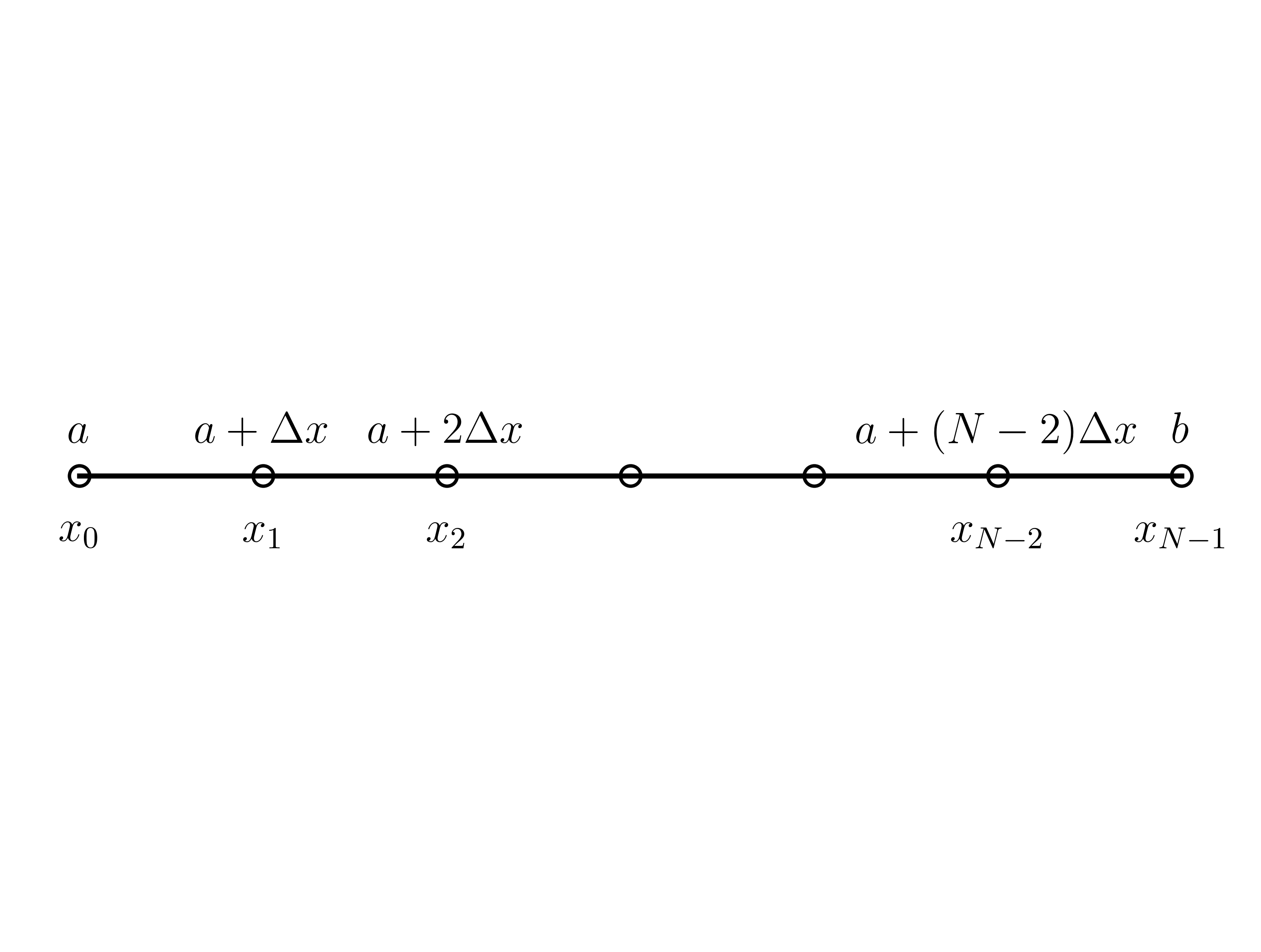
2.6.1. Spatial discretization

In a uniform grid, the \(i\)-th node in the grid is located at \(x_{i}=a+i\Delta x\).

\[ \Delta x= \dfrac{b-a}{N-1}. \]

x = np.arange(-3, 4)

fig, ax = plt.subplots()
ax.plot(x, np.zeros_like(x), "ko-", mfc="none")
ax.text(x[0], 0.004, rf"$a$", ha="center", fontsize=13)
ax.text(x[0], -0.008, rf"$x_0$", ha="center", fontsize=13)
ax.text(x[1], 0.004, rf"$a+\Delta x$", ha="center", fontsize=13)
ax.text(x[1], -0.008, rf"$x_1$", ha="center", fontsize=13)
ax.text(x[2], 0.004, rf"$a+2\Delta x$", ha="center", fontsize=13)
ax.text(x[2], -0.008, rf"$x_2$", ha="center", fontsize=13)
ax.text(x[-2], 0.004, rf"$a+(N-2)\Delta x$", ha="center", fontsize=13)
ax.text(x[-2], -0.008, rf"$x_{{N-2}}$", ha="center", fontsize=13)
ax.text(x[-1], 0.004, rf"$b$", ha="center", fontsize=13)
ax.text(x[-1], -0.008, rf"$x_{{N-1}}$", ha="center", fontsize=13)
ax.axes.get_xaxis().set_visible(False)
ax.axes.get_yaxis().set_visible(False)
ax.set_frame_on(False)

2.7. Deriving a finite-difference scheme

\[\begin{split} \begin{aligned} U_{t}+vU_{x}&=0\\ \dfrac{U^{n+1}_{i}-U^{n}_{i}}{\Delta t}+ v\dfrac{U^{n}_{i}-U^{n}_{i-1}}{\Delta x} &=0.\\ U^{n+1}_{i} &= U^{n}_{i}- \dfrac{v\Delta t}{\Delta x} \left(U^{n}_{i}-U^{n}_{i-1}\right). \end{aligned} \end{split}\]

v = symbols("v")

fig = plt.figure()
for i in range(4):
    plt.plot((0, 4), (i, i), "k")

for j in range(5):
    plt.plot((j, j), (0, 3), "k")

plt.plot(2, 2, "ko", mfc="none")
plt.plot(2, 1, "ko", mfc="none")
plt.plot(1, 1, "ko", mfc="none")

ax = fig.gca()
ax.axis("off")
ax.axis("equal")

plt.text(0.9, -0.15, "$i-1$", fontsize=12)
plt.text(2, -0.15, "$i$", fontsize=12)
plt.text(2.9, -0.15, "$i+1$", fontsize=12)
plt.text(2.1, 1.1, "$u^n_i$", fontsize=14)
plt.text(2.1, 2.1, "$u^{n+1}_i$", fontsize=14)
plt.text(1.05, 1.1, "$u^{n}_{i-1}$", fontsize=14)
plt.text(1.38, 0.85, r"$\Delta x$", fontsize=12)
plt.text(0.75, 1.45, r"$\Delta t$", fontsize=12)
plt.text(-0.35, 1, "$n$", fontsize=12)
plt.text(-0.35, 2, "$n+1$", fontsize=12)
plt.text(-0.35, 3, "Time")
plt.text(4, -0.15, "Space");

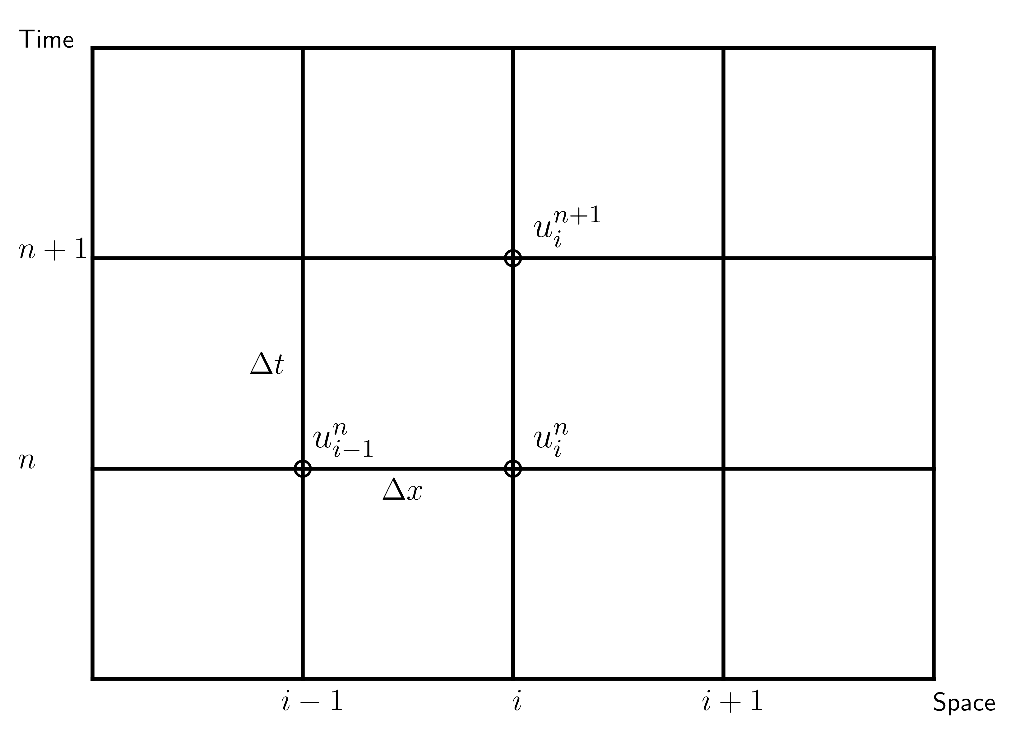
2.7.1. Computational and boundary nodes

t, x, a, b = symbols("t x a b")
U = Function("U")

Eq(U(t, a), 0)

\[\displaystyle U{\left(t,a \right)} = 0\]

Eq(U(t, b), 0)

\[\displaystyle U{\left(t,b \right)} = 0\]

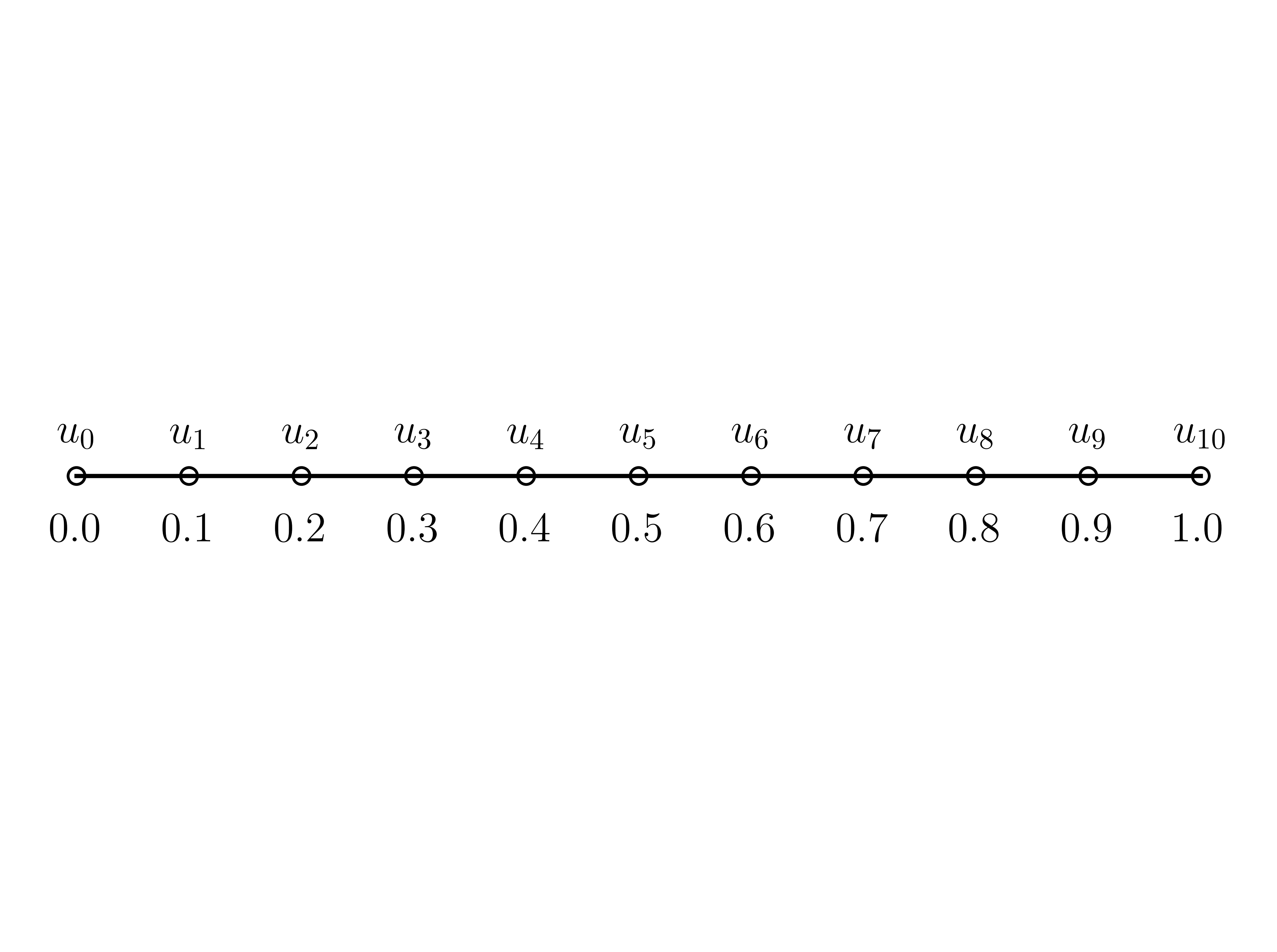
N = 11  # number of nodes
number_iterations = 3
x, dx = np.linspace(start=0, stop=1, num=N, retstep=True)  # node positions
v = 1  # speed
dt = 0.05  # time step
t = 0  # initial value of t

fig, ax = plt.subplots()
fig.set_tight_layout(True)
ax.plot(x, np.zeros_like(x), "ko-", mfc="none")
# ax.set_xlabel(r"$x_{i}$")
for i, xi in enumerate(x):
    ax.text(xi, 0.004, rf"$u_{{{i}}}$", ha="center", fontsize=15)
    ax.text(xi, -0.008, rf"${{{np.round(xi, 2)}}}$", ha="center", fontsize=15)
ax.axes.get_xaxis().set_visible(False)
ax.axes.get_yaxis().set_visible(False)
ax.set_frame_on(False)

C = v * dt / dx

U = np.empty((number_iterations + 1, x.size))
U[0, :] = np.exp(-100 * np.power(x - 0.4, 2))  # initial conditions
U[0, 0], U[0, -1] = (0, 0)

for n in range(number_iterations):
    U[n + 1, 0], U[n + 1, -1] = (0, 0)  # boundary nodes
    for i in range(x.size):
        U[n + 1, i] = U[n, i] - C * (U[n, i] - U[n, i - 1])

# Values of the first three iterations of the FDS used to solve the advection equation
tabular = np.hstack(
    (
        np.array(["i", "x_i", "u^0_i", "u^1_i", "u^2_i", "u^3_i"])[np.newaxis].T,
        np.vstack((np.arange(x.size)[np.newaxis], x, U)),
    )
)
print(tabulate(tabular, floatfmt=".4f"))

-----  ------  ------  ------  ------  ------  ------  ------  ------  ------  ------  -------
i      0.0000  1.0000  2.0000  3.0000  4.0000  5.0000  6.0000  7.0000  8.0000  9.0000  10.0000
x_i    0.0000  0.1000  0.2000  0.3000  0.4000  0.5000  0.6000  0.7000  0.8000  0.9000   1.0000
u^0_i  0.0000  0.0001  0.0183  0.3679  1.0000  0.3679  0.0183  0.0001  0.0000  0.0000   0.0000
u^1_i  0.0000  0.0001  0.0092  0.1931  0.6839  0.6839  0.1931  0.0092  0.0001  0.0000   0.0000
u^2_i  0.0000  0.0000  0.0046  0.1012  0.4385  0.6839  0.4385  0.1012  0.0046  0.0000   0.0000
u^3_i  0.0000  0.0000  0.0023  0.0529  0.2698  0.5612  0.5612  0.2698  0.0529  0.0023   0.0000
-----  ------  ------  ------  ------  ------  ------  ------  ------  ------  ------  -------

with np.printoptions(precision=5, suppress=True):
    print(np.array([np.pi]))

[3.14159]