Numerical integration: Part II

57. Numerical integration: Part II#

Anne Kværnø, André Massing

Date: Jan 28, 2021

import matplotlib.pyplot as plt
import numpy as np
from IPython.core.display import HTML
from numpy import pi


def css_styling():
    try:
        with open("tma4125.css") as f:
            styles = f.read()
            return HTML(styles)
    except FileNotFoundError:
        pass  # Do nothing


# Comment out next line and execute this cell to restore the default notebook style
css_styling()

As usual, we import the necessary modules before we get started.

%matplotlib inline

newparams = {
    "figure.figsize": (8.0, 4.0),
    "axes.grid": True,
    "lines.markersize": 8,
    "lines.linewidth": 2,
    "font.size": 14,
}
plt.rcParams.update(newparams)

58. General construction of quadrature rules#

In the following, you will learn the steps on how to construct realistic algorithms for numerical integration, similar to those used in software like Matlab of SciPy. The steps are:

Construction.

Choose $n + 1$ distinct nodes on a standard interval $I$ , often chosen to be $I = [- 1, 1]$ .
Let $p_{n} (x)$ be the polynomial interpolating some general function $f$ in the nodes, and let the $Q [f] (- 1, 1) = I [p_{n}] (- 1, 1)$ .
Transfer the formula $Q$ from $[- 1, 1]$ to some interval $[a, b]$ .
Design a composite formula, by dividing the interval $[a, b]$ into subintervals and applying the quadrature formula on each subinterval.
Find an expression for the error $E [f] (a, b) = I [f] (a, b) - Q [f] (a, b)$ .
Find an expression for an estimate of the error, and use this to create an adaptive algorithm.

In this course, we will not have the time to cover the last two steps.

59. Constructing quadrature rules on a single interval#

We have already seen in the previous Lecture how quadrature rules on a given interval $[a, b]$ can be constructed using polynomial interpolation.

For $n + 1$ quadrature points ${x_{i}}_{i = 0}^{n} \subset [a, b]$ , we compute weights by

w_{i} = \int_{a}^{b} ℓ_{i} (x) d x for i = 0, \dots, n .

where $ℓ_{i} (x)$ are the cardinal functions associated with ${x_{i}}_{i = 0}^{n}$ satisfying $ℓ_{i} (x_{j}) = δ_{i j}$ for $i, j = 0, 1, \dots, n$ . The resulting quadrature rule has (at least) degree of exactness equal to $n$ .

But how to you proceed if you know want to compute an integral on a different interval, say $[c, d]$ ? Do we have to reconstruct all the cardinal functions and recompute the weights?

The answer is NO! One can easily transfer quadrature points and weights from one interval to another. One typically choose the simple reference interval $\hat{I} = [- 1, 1]$ . Then you determine some $n + 1$ quadrature points ${{\hat{x}}_{i}}_{i = 0}^{n} \subset [- 1, 1]$ and quadrature weights ${{\hat{w}}_{i}}_{i = 0}^{n}$ to define a quadrature rule $Q (\hat{I})$

The quadrature points can then be transferred to an arbitrary interval $[a, b]$ to define a quadrature rule $Q (a, b)$ using the transformation

x = \frac{b - a}{2} \hat{x} + \frac{b + a}{2}, so d x = \frac{b - a}{2} d \hat{x},

and thus we define ${x_{i}}_{i = 0}^{n}$ and ${w_{i}}_{i = 0}^{n}$ by

x_{i} = \frac{b - a}{2} {\hat{x}}_{i} + \frac{b + a}{2}, w_{i} = \frac{b - a}{2} {\hat{w}}_{i} for i = 0, \dots n .

59.1. Example 1: Simpson’s rule#

Choose standard interval $[- 1, 1]$ . For Simpson’s rule, choose the nodes $t_{0} = - 1$ , $t_{1} = 0$ and $t_{2} = 1$ . The corresponding cardinal functions are
- $ℓ_{0} = \frac{1}{2} (t^{2} - t), ℓ_{1} (t) = 1 - t^{2}, ℓ_{2} (t) = \frac{1}{2} (t^{2} + t)$ .
which gives the weights
- $w_{0} = \int_{- 1}^{1} ℓ_{0} (t) d t = \frac{1}{3}, w_{1} = \int_{- 1}^{1} ℓ_{1} (t) d t = \frac{4}{3}, w_{2} = \int_{- 1}^{1} ℓ_{2} (t) d t = \frac{1}{3}$
such that
- $\int_{- 1}^{1} f (t) d t \approx \int_{- 1}^{1} p_{2} (t) d t = \sum_{i = 0}^{2} w_{i} f (t_{i}) = \frac{1}{3} [f (- 1) + 4 f (0) + f (1)]$ .
After transferring the nodes and weights, Simpson’s rule over the interval $[a, b]$ becomes
- $S (a, b) = \frac{b - a}{6} [f (a) + 4 f (c) + f (b)], c = \frac{b + a}{2}$ .

60. Composite quadrature rules#

To generate more accurate quadrature rule $Q (a, b)$ we have in principle two possibilities:

Increase the order of the interpolation polynomial used to construct the quadrature rule.

Subdivide the interval $[a, b]$ into smaller subintervals and apply a quadrature rule on each of the subintervals, leading to Composite Quadrature Rules which we will consider next.

Select $m ⩾ 2$ and divide $[a, b]$ into $m$ equally spaced subintervals $[x_{i - 1}, x_{i}]$ defined by $x_{i} = a + i h$ with $h = (b - a) / m$ for $i = 1, \dots, m$ . Then for a given quadrature rule $Q [\cdot] (x_{i - 1}, x_{i})$ the corresponding composite quadrature rule $CQ [\cdot] ({[x_{i - 1}, x_{i}]}_{i = 1}^{m})$ is given by

\begin{matrix} (1) & \int_{a}^{b} f d x \approx CQ [f] ({[x_{i - 1}, x_{i}]}_{i = 1}^{m}) = \sum_{i = 1}^{m} Q [f] (x_{i - 1}, x_{i}) . \end{matrix}

60.1. Composite trapezoidal rule#

Using the trapezoidal rule $T [f] (x_{i - 1}, x_{i}) = \frac{h}{2} f (x_{i - 1}) + \frac{h}{2} f (x_{i})$ the resulting composite trapezoidal rule is given by

\begin{array}{r} \int_{a}^{b} f d x \approx CT [f] ({[x_{i - 1}, x_{i}]}_{i = 1}^{m}) = h [\frac{1}{2} f (x_{0}) + f (x_{1}) + \dots + f (x_{m - 1}) + \frac{1}{2} f (x_{m})] \end{array}

60.2. Exercise 1: Testing the accuracy of the composite trapezoidal rule#

Have a look at the CT function which implements the composite trapezoidal rule:

def CT(f, a, b, m):
    """Computes an approximation of the integral f
    using the composite trapezoidal rule.
    Input:
        f:  integrand
        a:  left interval endpoint
        b:  right interval endpoint
        m:  number of subintervals
    """
    x = np.linspace(a, b, m + 1)
    h = float(b - a) / m
    fx = f(x[1:-1])
    ct = h * (np.sum(fx) + 0.5 * (f(x[0]) + f(x[-1])))
    return ct

Use this function to compute an approximate value of integral

I (0, 1) = \int_{0}^{1} \cos (\frac{π}{2} x) = \frac{2}{π} = 0.636619 \dots .

for $m = 4, 8, 16, 32, 64$ corresponding to $h = 2^{- 2}, 2^{- 3}, 2^{- 4}, 2^{- 5}, 2^{- 6}$ . Tabulate the corresponding quadrature errors $I (0, 1) - Q (0, 1)$ . What do you observe?

# Insert your code here.

Solution.

# Define function


def f(x):
    return np.cos(pi * x / 2)


# Exact integral
int_f = 2 / pi

# Interval
a, b = 0, 1

# Compute integral numerically
for m in [4, 8, 16, 32, 64]:
    cqr_f = CT(f, a, b, m)
    print(f"Number of subintervals m = {m}")
    print(f"Q[f] = {cqr_f}")
    print(f"I[f] - Q[f] = {int_f - cqr_f:.10e}")

Number of subintervals m = 4
Q[f] = 0.6284174365157311
I[f] - Q[f] = 8.2023358519e-03
Number of subintervals m = 8
Q[f] = 0.6345731492255537
I[f] - Q[f] = 2.0466231420e-03
Number of subintervals m = 16
Q[f] = 0.6361083632808496
I[f] - Q[f] = 5.1140908673e-04
Number of subintervals m = 32
Q[f] = 0.6364919355013015
I[f] - Q[f] = 1.2783686628e-04
Number of subintervals m = 64
Q[f] = 0.636587814113642
I[f] - Q[f] = 3.1958253939e-05

60.2.1. Remarks#

We observe that for each doubling of the number of subintervals we decrease the error by a fourth. That means that if we look at the quadrature error $I [f] - CT [f]$ as a function of the number of subintervals $m$ (or equivalently as a function of $h$ ), then $| I [f] - CT [f] | \approx \frac{C}{m^{2}} = C h^{2}$ .

60.3. Error estimate for the composite trapezoidal rule#

We will now theoretically explain the experimentally observed convergence rate in the previous Exercise 1: Testing the accuracy of the composite trapezoidal rule.

First we have to recall the error estimate for for the trapezoidal rule on a single interval $[a, b]$ . If $f \in C^{2} (a, b)$ , then there is a $ξ \in (a, b)$ such that

I [f] - T [f] = \frac{(b - a)^{3}}{12} f^{″} (ξ) .

60.4. Theorem 1: Quadrature error estimate for composite trapezoidal rule#

Let $f \in C^{2} (a, b)$ , then the quadrature error $I [f] - CT [f]$ for the composite trapezoidal rule can be estimated by

\begin{matrix} (2) & | I [f] - CT [f] | ⩽ \frac{M_{2}}{12} \frac{(b - a)^{3}}{m^{2}} = \frac{M_{2}}{12} h^{2} (b - a) \end{matrix}

where $M_{2} = max_{ξ \in [a, b]} | f^{″} (ξ) |$ .

Proof.

\begin{array}{r} \begin{aligned} | I [f] - CT [f] | & = | \sum_{i = 1}^{m} [\int_{x_{i - 1}}^{x_{i}} f (x) d x - (\frac{h}{2} f (x_{i - 1}) + \frac{h}{2} f (x_{i}))] | \\ ⩽ \sum_{i = 1}^{m} \frac{h^{3}}{12} | f^{″} (ξ_{i}) | ⩽ M_{2} \sum_{i = 1}^{m} \frac{(h)^{3}}{12} \\ = M_{2} \frac{h^{3}}{12} \underset{\frac{(b - a)}{h}}{\underset{⏟}{m}} = \frac{M_{2}}{12} h^{2} (b - a) = \frac{M_{2}}{12} \frac{(b - a)^{3}}{m^{2}} \end{aligned} . \end{array}

60.5. Interlude: Convergence of $h$ -dependent approximations#

Let $X$ be the exact solution, and $X (h)$ some numerical solution depending on a parameter $h$ , and let $e (h)$ be the norm of the error, so $e (h) = ‖ X - X (h) ‖$ . The numerical approximation $X (h)$ converges to $X$ if $e (h) \to 0$ as $h \to 0$ . The order of the approximation is $p$ if there exists a positive constant $M$ such that $ $e (h) \leq M h^{p}$ $

The Big $O$ -notation we can simply write $ $e (h) = O (h^{p}) as h \to 0.$ $T h i s i s o f t e n u s e d w h e n w e a r e n o t d i r e c t l y i n t e r e s t e d i n a n y e x p r e s s i o n f o r t h e c o n s t a n t$ M$, we only need to know it exists.

Again, we see that a higher approximation order $p$ leads for small values of $h$ to a better approximation of the solution. Thus we are generally interested in approximations of higher order.

60.5.1. Numerical verification#

The following is based on the assumption that $e (h) \approx C h^{p}$ for some unknown constant $C$ . This assumption is often reasonable for sufficiently small $h$ .

Choose a test problem for which the exact solution is known and compute the error for a decreasing sequence of $h_{k}$ ’s, for instance $h_{k} = H / 2^{k}$ , $k = 0, 1, 2, \dots$ . The procedure is then quite similar to what was done for iterative processes.

\begin{array}{r} \begin{array}{rcl} e (h_{k + 1}) & \approx & C h_{k + 1}^{p} \\ e (h_{k}) & \approx & C h_{k}^{p} \end{array} \Rightarrow \frac{e (h_{k + 1})}{e (h_{k})} \approx {(\frac{h_{k + 1}}{h_{k}})}^{p} \Rightarrow p \approx \frac{\log (e (h_{k + 1}) / e (h_{k}))}{\log (h_{k + 1} / h_{k})} \end{array}

For one refinement step where one passes from $h_{k} \to h_{k + 1}$ , the number $ $E O C (k) \approx \frac{\log (e (h_{k + 1}) / e (h_{k}))}{\log (h_{k + 1} / h_{k})}$ $ is often called the “Experimental order of convergence at refinement level k”

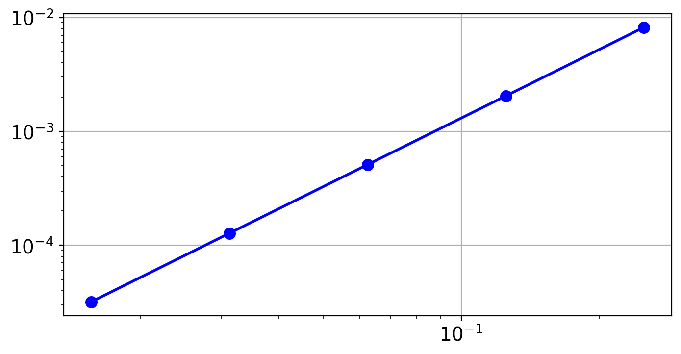
Since $ $e (h) \approx C h^{p} \Rightarrow \log e (h) \approx \log C + p \log h$ $a p l o t o f$ e(h) $a s a f u n c t i o n o f$ h $u s i n g a l o g a r i t h m i c s c a l e o n b o t h a x e s (a l o g - l o g p l o t) w i l l b e a s t r a i g h t l i n e w i t h s l o p e$ p$. Such a plot is referred to as an error plot or a convergence plot.

60.6. Exercise 1 (extension): Examine the convergence order of composite trapezoidal rule#

# Insert your code here.

Solution

# Define function


def f(x):
    return np.cos(pi * x / 2)


# Exact integral
int_f = 2 / pi

# Interval
a, b = 0, 1

errs = []
hs = []

# Compute integral numerically
for m in [4, 8, 16, 32, 64]:
    cqr_f = CT(f, a, b, m)
    print(f"Number of subintervals m = {m}")
    print(f"Q[f] = {cqr_f}")
    err = int_f - cqr_f
    errs.append(err)
    hs.append((b - a) / m)
    print(f"I[f] - Q[f] = {err:.10e}")

hs = np.array(hs)
errs = np.array(errs)
eoc = np.log(errs[1:] / errs[:-1]) / np.log(hs[1:] / hs[:-1])
print(eoc)
plt.loglog(hs, errs, "bo-")

Number of subintervals m = 4
Q[f] = 0.6284174365157311
I[f] - Q[f] = 8.2023358519e-03
Number of subintervals m = 8
Q[f] = 0.6345731492255537
I[f] - Q[f] = 2.0466231420e-03
Number of subintervals m = 16
Q[f] = 0.6361083632808496
I[f] - Q[f] = 5.1140908673e-04
Number of subintervals m = 32
Q[f] = 0.6364919355013015
I[f] - Q[f] = 1.2783686628e-04
Number of subintervals m = 64
Q[f] = 0.636587814113642
I[f] - Q[f] = 3.1958253939e-05
[2.00278934 2.00069577 2.00017385 2.00004346]

[<matplotlib.lines.Line2D at 0x7fee1892c680>]

../_images/64169a57fc7a5aac855437112ca78d1466e25ebf46cb9d5ff406ca5f42cf6fef.png

60.7. Exercise 2: Composite Simpson’s rule#

We can now play the exact same game to construct and analyze a Composite Simpson’s rule. In this set of exercises you are ask to develop the code and theory for the composite Simpson’s rule. This will be part of the next homework assignment.

a) Start from Simpson’s rule

S [f] (x_{i - 1}, x_{i}) = \frac{h}{6} (f (x_{x_{i - 1}}) + 4 f (x_{i - 1 / 2}) + f (x_{i})),

where $x_{i - 1 / 2} = \frac{x_{i - 1} + x_{i}}{2}$ is the midpoint of the interval $[x_{i - 1}, x_{i}]$ .

Show that the resulting composite Simpson’s rule is given by

\begin{array}{r} \begin{aligned} \int_{a}^{b} f d x \approx CSR [f] ({[x_{i}, x_{i + 1}]}_{i = 1}^{m}) & = \frac{h}{6} [f (x_{0}) + 4 f (x_{x_{1 / 2}}) + 2 f (x_{1}) + 4 f (x_{3 / 2}) + 2 f (x_{2}) + \dots \\ + 2 f (x_{m - 1}) + 4 f (x_{x_{m - 1 / 2}}) + f (x_{m})] . \end{aligned} \end{array}

b) Implement the composite Simpson’s rule. Use this function to compute an approximate value of integral

I (0, 1) = \int_{0}^{1} \cos (\frac{π}{2} x) = \frac{2}{π} = 0.636619 \dots .

for $m = 4, 8, 16, 32, 64$ corresponding to $h = 2^{- 2}, 2^{- 3}, 2^{- 4}, 2^{- 5}, 2^{- 6}$ . Tabulate the corresponding quadrature errors $I (0, 1) - Q (0, 1)$ . What do you observe? How does it compare to the composite trapezoidal rule?

# Insert your code here.

c) Recall the error estimate for Simpson’s rule on a single interval, stating that there is a $ξ \in (a, b)$ such that

I [f] - Q [f] = - \frac{(b - a)^{5}}{2880} f^{4} (ξ) .

whenever $f \in C^{4} (a, b)$ . Start from this estimate and prove the following theorem.

60.8. Theorem 2: Quadrature error estimate for composite Simpon’s rule#

Let $f \in C^{4} (a, b)$ , then the quadrature error $I [f] - CT [f]$ for the composite trapezoidal rule can be estimated by

\begin{matrix} (3) & | I [f] - CSR [f] | \leq \frac{M_{4}}{2880} \frac{(b - a)^{5}}{m^{4}} = \frac{M_{4}}{2880} h^{4} (b - a) \end{matrix}

where $M_{4} = max_{ξ \in [a, b]} | f^{(4)} (ξ) |$ .