53.1. Introduction#

In this note the finite difference method for solving partial differential equations (PDEs) will be presented.

Roughly speaking, a finite difference method consists of the following steps:

1. Discretize the domain on which the equation is defined.

2. On each grid point, replace the derivatives with an approximation, using the values in neighbouring grid points.

3. Replace the exact solutions by their approximations.

4. Solve the resulting system of equations.

We will first see how to find approximations to the derivative of a function, and then how these can be used to solve boundary value problems like

and time dependent partial differential equations like the heat equation

The technique described here is, however, applicable to several other PDEs, and it is therefore important to try to understand the underlying idea.

53.2. Numerical differentiation#

This is the main tool for finite difference methods.

Given a sufficiently smooth function $u$. How can we find an approximation to $u^{\prime }(x)$ or $u^{″}(x)$ in some given point $x$, just by using evaluation of the function itself?

The derivative of $u$ is defined as

Given a sufficiently small value of $h$, the right hand side can be used an approximation to the first derivative $u^{\prime }(x)$. A small collection of the most used approximations to the first order derivative $u^{\prime }(x)$ is:

The first one is taken directly from the definition, and so is the second, and the third is just the mean of the first two.

A common approximation to the second derivative is

Numerical example 1: Test the method on the function $u(x)=\sin (x)$ at the point $x=\frac{\pi }{4}$. Compare with the exact derivative. Try different step sizes, e.g. $h=0.1,h=0.01,h=0.001$. Notice how the error in each case changes with $h$.

import matplotlib.pyplot as plt
import numpy as np

# Import linear algebra module
import scipy.linalg as la
from matplotlib import cm
from matplotlib.pyplot import *
from mpl_toolkits.mplot3d import Axes3D  # For 3-d plot
from numpy import *
from scipy.linalg import solve  # Solve linear systems
from scipy.sparse import diags  # Greate diagonal matrices

%matplotlib inline

newparams = {
    "figure.figsize": (8.0, 4.0),
    "axes.grid": True,
    "lines.markersize": 8,
    "lines.linewidth": 2,
    "font.size": 14,
}
rcParams.update(newparams)

# Numerical differentiation

# Forward difference


def diff_forward(u, x, h=0.1):
    return (u(x + h) - u(x)) / h


# Backward difference


def diff_backward(u, x, h=0.1):
    return (u(x) - u(x - h)) / h


# Central difference for f'(x):


def diff_central(u, x, h=0.1):
    return (u(x + h) - u(x - h)) / (2 * h)


# end of diff_central

# Central difference for f''(x):


def diff2_central(u, x, h=0.1):
    return (u(x + h) - 2 * u(x) + u(x - h)) / h**2


# end of diff2_central

# Numerical example 1
x = pi / 4
du_exact = cos(x)
ddu_exact = -sin(x)
for h in [0.1, 0.01, 0.001]:
    u = sin
    du = diff_forward(u, x, h)
    print(f"Approximations to the first derivative for h = {h}")
    print(f"Forward difference:  du  = {du:12.8f},  Error = {du_exact-du:10.3e}")
    du = diff_backward(u, x, h)
    print(f"Backward difference: du  = {du:12.8f},  Error = {du_exact-du:10.3e}")
    du = diff_central(u, x, h)
    print(f"Central difference:  du  = {du:12.8f},  Error = {du_exact-du:10.3e}")
    print("Approximation to the second derivative")
    ddu = diff2_central(u, x, h)
    print(f"Central difference:  ddu = {ddu:12.8f}, Error = {ddu_exact-ddu:10.3e}")

Approximations to the first derivative for h = 0.1
Forward difference:  du  =   0.67060297,  Error =  3.650e-02
Backward difference: du  =   0.74125475,  Error = -3.415e-02
Central difference:  du  =   0.70592886,  Error =  1.178e-03
Approximation to the second derivative
Central difference:  ddu =  -0.70651772, Error = -5.891e-04
Approximations to the first derivative for h = 0.01
Forward difference:  du  =   0.70355949,  Error =  3.547e-03
Backward difference: du  =   0.71063050,  Error = -3.524e-03
Central difference:  du  =   0.70709500,  Error =  1.179e-05
Approximation to the second derivative
Central difference:  ddu =  -0.70710089, Error = -5.893e-06
Approximations to the first derivative for h = 0.001
Forward difference:  du  =   0.70675311,  Error =  3.537e-04
Backward difference: du  =   0.70746022,  Error = -3.534e-04
Central difference:  du  =   0.70710666,  Error =  1.179e-07
Approximation to the second derivative
Central difference:  ddu =  -0.70710672, Error = -5.901e-08

53.3. Error analysis#

In this case the error analysis is quite simple: Perform a Taylor expansion of the error around $x$. The Taylor expansion becomes a power series in $h$.

The expansion for the error of the forward difference is:

\begin{align*} e(x;h) &= u’(x) - \frac{u(x+h)-u(x)}{h} \ &= u’(x) - \frac{(u(x)+u’(x)h + \frac{1}{2}u’’(\xi)h^2) - u(x)}{h} \ &= -\frac{1}{2}u’’(\xi)h \end{align*}

for some $\xi \in (x,x+h)$.

The expansion for the error of the central difference is slightly more complicated:

\begin{align*} e(x; h) &= u’(x) - \frac{u(x+h)-u(x-h)}{2h} \ &= u’(x) \ &- \frac{\big(u(x)+u’(x)h + \frac{1}{2} u’’(x)h^2 + \frac{1}{6} u’’’(\xi_1)h^3 \big) - \big(u(x)-u’(x)h + \frac{1}{2} u’’(x)h^2 - \frac{1}{6} u’’’(\xi_2)h^3\big)}{2h} \ &= -\frac{1}{12}\big(u’’’(\xi_1) + u’’’(\xi_2)\big)h^2 \ &= -\frac{1}{6}u’’’(\eta)h^2, \qquad \qquad \text{ for some } \eta \in (x-h, x+h). \end{align*}

In the last step, the two remainder terms have been combined by the intermediate value theorem. The error for the approximation of the second order derivative can be found in a similar manner.

Problem 1: Use Taylor expansion to show that for $u\in C^4([a,b])$

Reminder. The order of an approximation is $p$ if there exist a constant $C$ independent on $h$ such that

for all sufficiently small $h>0$.

In practice, it is sufficient to show that the power expansion of the error satisfies

The forward and backward approximations are of order 1, the central differences of order 2.

We are going to use these formulas a lot in the sequel, so let us just summarize the results, including the error terms:

Difference formulas for derivatives:

\begin{align*} u’(x) &= \left{ \begin{array}{ll} \displaystyle \underbrace{\frac{u(x+h)-u(x)}{h}}{\partial^+u(x)} - \frac{h}{2}u’’(\xi), \ & \text{Forward difference} \ \mbox{} \ \displaystyle \underbrace{\frac{u(x)-u(x-h)}{h}}{\partial^-u(x)} + \frac{h}{2}u’’(\xi), & \text{Backward difference} \ \mbox{} \ \displaystyle \underbrace{\frac{u(x+h)-u(x-h)}{2h}}{\partial^{\circ}u(x)} - \frac{h^2}{6}u’’’(\xi).\qquad & \text{Central difference} \end{array} \right. \ \mbox{} \ u’’(x) & = \underbrace{\frac{u(x+h)-2u(x)+u(x-h)}{h^2}}{\partial^+\partial^-u(x)} - \frac{h^2}{12}u^{(4)}(\xi), \qquad
\text{Central difference} \end{align*}

53.4. Finite difference method for the 1d Poisson problem#

We start our journey with the the following problem. Let $[a,b]\subset \mathbb{R}$ be a finite interval, together with a function $f:[a,b]\to \mathbb{R}$. Then the two-point boundary value problem is to find a $u:[a,b]\to \mathbb{R}$ such that

\begin{gather}

• u’’(x) = f(x) \quad \forall x \in (a,b), \tag{1a} \ u(a) = u_a, \quad u(b) = u_b \tag{1b} \end{gather} where $u_a$ and $u_b$ are given values.

For the rest of the this section we will assume that $a=0,b=1$

Note that so this is second order ordinary differential equations and thus requires two addition values to determine a solution completely, one on each boundary point.

This is contrast of the second order initial value problem \begin{align*} u’’ &= f(t,u(t), u’(t)) \quad \forall; t \in (0,1) \ u(0) &= u_0, \ u’(0) &= u_1 \end{align*} where we have two conditions on the left end point. The main reason is that in the former case, $x$ is a space variable, while in the latter case, $t$ is a time variable.

Instead of trying to compute $u(x)$ exactly, we will now try to compute a numerical approximation $u_{\mathrm{\Delta }}$ of $u(x)$. As many times before we start by defininig $n+1$ equally spaced points $\{x_i{\}}_{i=0}^n$ with a grid size $h=\frac{b-a}{n}$ so that $$x_i:=a+ih\text{for }i=0,1,\dots ,n.$$

Then the second order derivative $u^{″}$ can be approximated by the central difference operator defined by

\begin{align} \partial^+ \partial^- u(x_i) := \dfrac{u(x_i+h) - 2 u(x_i) + u(x_i-h)} {h^2} \approx u’’(x_i) = -f(x_i) \end{align}

Now the idea is to numerically solve for the two-point boundary value problem by associating an unknown variable $U_i:=u_{\mathrm{\Delta }}(x_i)$ to every grid point $x_i$ for $i=0,\dots N$. Of course, the goal is to find an $U_i\approx u(x_i)$. Keeping in mind that $-u^{″}=f$, we demand that at the internal grid points $\{x_i{\}}_{i=1}^N$ the unknows satisfy

56.1. Implementation#

def fdm_poisson1d_matrix(N):
    r"""Computes the finite difference matrix for the Poisson problem in 1D

    Parameters:
    N (int): Number of grid points :math:`\{x_i}_{i=0}^N` counting from 0.

    Returns:
    A (ndarray): Finite difference matrix

    """
    # Gridsize
    h = 1.0 / N

    # Define zero matrix A of right size and insert
    A = np.zeros((N + 1, N + 1))

    # Define tridiagonal part of A
    hh = h * h
    for i in range(1, N):
        A[i, i - 1] = -1 / hh
        A[i, i] = 2 / hh
        A[i, i + 1] = -1 / hh

    # Set a_00 = a_NN to 1 to incorporate boundary condition
    A[0, 0] = 1
    A[N, N] = 1

    return A


def apply_bcs(F, bcs):
    "Incorporate boundary condition into rhs vector"
    F[0], F[-1] = bcs[0], bcs[1]

# Analytical reference solution
u = lambda x: np.sin(2 * np.pi * x)
f = lambda x: (2 * np.pi) ** 2 * np.sin(2 * np.pi * x)

N = 10

# Define grid points
x = np.linspace(0, 1, N + 1)
xfine = np.linspace(0, 1, 10 * N)

# Compute A and F
A = fdm_poisson1d_matrix(N)
F = f(x)
# print(A)
# print(F)

# Incorporate bcs
bcs = [u(0), u(1)]
apply_bcs(F, bcs)

# Solve AU = F
# (We will introduce a sparse solver when we look at 2D problems)
U = la.solve(A, F)

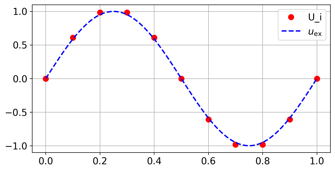
# Plot discrete solution on chosen discretization grid
plt.plot(x, U, "or", label="U_i")
plt.plot(xfine, u(xfine), "--b", label=r"$u_{\mathrm{ex}}$")
plt.legend()
# Show figure (for non inline plotting)
plt.show()

Problem 2

Apply the method of manufactured solutions: Take a known function $u(x)$ and compute corresponding data $f$ and $u_a$, $u_b$ such that $u$ is the solution to the two-point two-point boundary problem (1a)–(1b).

For example you can pick $u(x)=\cos (2\pi x)$. What is then $f=-u^{″}$, $u_a=u(0)$, $u_b=u(1)$?

After having picked your favorite (smooth) manufactured solution, you can compute the error $$\mathrm{err}(\mathrm{h})=\mathrm{err}(\mathrm{N})=\underset{i\in \{0,\dots N\}}{max}|U_i-u(x_i)|$$asafunctionof$h = 1/N$.

For $N_1=5,N_2=10,N_3=20,N_4=40,N_5=80$

• compute and plot the numerical solution and the analytical solution

• record the resulting $\mathrm{err}(\mathrm{N})$

At the end of your experiment, compute the experimental order of convergence for each refinement level $N_2,\dots ,N_5$ defined $$EOC(N_i)={\displaystyle \frac{\log (\mathrm{err}(N_i))-\log (\mathrm{err}(N_{i-1}))}{\log (N_{i-1})-\log (N_i)}}$$

What order of convergence do you expect and what do you get?

56.2. General two point boundary problems (BVP)#

In the following, we will discuss the numerical solution of a two-point boundary value problem of the form

where $p$, $q$ are given functions of $x$ and the boundary values $u_a$ and $u_a$ are given constants.

As before, a finite difference method for this problem is constructed with the following steps:

Step 1: Given the interval $[a,b]$. Choose some $N\in \mathbb{N}$, define the step size $h=(b-a)/N$, and the grid points $x_i=a+ih$, $i=0,1,\dots ,N$.

Step 2: For each interior grid point $x_i$, $i=1,\dots ,N-1$, replace the derivatives by their approximations in the BVP. The result is:

for each $i=1,2\dots ,N-1$, and the term $\mathcal{O}(h^2)$ represents the errors in the difference formulas.

Step 3: Ignore the error term, and replace the exact solution $u(x_i)$ by its numerical (and still unknown) approximation $U_i$:

This is the discretization of the BVP.

If we now include the two boundary values as equations

the discretization is a linear system of equations

where $A$ is an $(N+1)\times (N+1)$ matrix and $\mathbf{U}=[U_0,\dots ,U_N{]}^T$. Or more specific, by multiplying the equations by $h^2$ we end up with:

The right hand side $\mathbf{b}$ is given by

Obviously, the first and last equations are trivial to solve, and are therefore often included in the right hand side.

Step 4: Solve $A\mathbf{U}=\mathbf{b}$ with respect to $\mathbf{U}$.

Example 1: We consider the equation

with exact solution $u(x)=e^{-3x}+2e^x-3x-2$.

Choose $N$, let $h=1/N$. Use the central differences for $u^{\prime }$ and $u^{″}$, such that

Let $U_i\approx u(x_i)$. Multiply by $h^2$ on both sides, include $U_0=u_a$ og $U_N=u_b$ and clean the mess:

\begin{align*} U_0 &= 1, \ (1-h)U_{i-1} + (-2-3h^2)U_i + (1+h)U_{i+1} &= 9x_ih^2, && i=1, \ldots, N-1, \ U_N &= 0.486351. \end{align*}

To be even more concrete, for $N=4$, we get $h=0.25$. The linear system of equations becomes

The first and the last equation is trivial to solve, so in practice you have a system of 3 equations in 3 unknowns,

with the solution

For comparison, the analytic solution in these points is

56.3. Implementation#

For simplicity, the implementation below is only done for BVPs with constant coefficients, that is $p(x)=p$ and $q(x)=q$. This makes the diagonal, sub- and super-diagonals constant, except at the first and the last row.
An extra function is included to construct tridiagonal matrices, that is, matrices where all entries outside the diagonal, sub-diagonal, and super-diagonal are equal to zero.

The implementation consist of:

1. Choose $N$, let $h=(b-a)/N$ and $x_i=a+ih$, $i=0,\dots ,N$.

2. Construct the matrix $A\in {\mathbb{R}}^{(N+1)\times (N+1)}$ and the vector $b\in {\mathbb{R}}^{N+1}$. The matrix $A$ is tridiagonal, and except from the first and last row, has the elements $v=1-\frac{h}{2}p$ below the diagonal, $d=-2+h^{2}q$ as diagonal elements and $w=1+\frac{h}{2}p$ above the diagonal.

3. Construct the vector $\mathbf{b}=[b_0,\dots ,b_N{]}^T$ with elements $b_i=h^{2}r(x_i)$ for $i=1,\dots ,N-1$.

4. Modify the first and the last row of the matrix $A$ and the first and last element of the vector $\mathbf{b}$, depending on the boundary conditions.

5. Solve the system $A\mathbf{U}=\mathbf{b}$.

def tridiag(v, d, w, N):
    """
    Help function
    Returns a tridiagonal matrix A=tridiag(v, d, w) of dimension N x N.
    """

    e = ones(N)  # array [1,1,...,1] of length N
    A = v * diag(e[1:], -1) + d * diag(e) + w * diag(e[1:], 1)
    return A

diag?

# Example 1, BVP

# Define the equation
# u'' + p*u' + q*u = r(x) on the interval [a,b]
# Boundary condition: u(a)=ua and u(b)=ub

p = 2
q = -3


def r(x):
    return 9 * x


a, b = 0, 1
ua, ub = 1, exp(-3) + 2 * exp(1) - 5

# The exact solution (if known)


def u_eksakt(x):
    return exp(-3 * x) + 2 * exp(x) - 3 * x - 2


# Set up the discrete system
N = 4  # Number of intervals

# Start the discretization
h = (b - a) / N  # Stepsize
x = linspace(a, b, N + 1)  # The gridpoints x_0=a, x_1=a+h, .... , x_N=b

# Make a draft of the A-matrix (first and last row have to be adjusted)
v = 1 - 0.5 * h * p  # Subdiagonal
d = -2 + h**2 * q  # Diagonal
w = 1 + 0.5 * h * p  # Superdiagonal
A = tridiag(v, d, w, N + 1)

# Make a draft of the b-vector
b = h**2 * r(x)

# Modify the first equation (left boundary)
A[0, 0] = 1
A[0, 1] = 0
b[0] = ua

# Modify the last equation (right boundary)
A[N, N] = 1
A[N, N - 1] = 0
b[N] = ub


U = solve(A, b)  #  Solve the equation

To verify the calculations done above, print the matrix $A$, the vector $\mathbf{b}$ and the numerical solution $\mathbf{U}$.

# Print the matrix A, the right hand side b the numerical and exact solution
print("A =\n", A)
print("\nb =\n ", b)
print("\nU =\n ", U)
print("\nu(x)=\n", u_eksakt(x))

A =
 [[ 1.      0.      0.      0.      0.    ]
 [ 0.75   -2.1875  1.25    0.      0.    ]
 [ 0.      0.75   -2.1875  1.25    0.    ]
 [ 0.      0.      0.75   -2.1875  1.25  ]
 [ 0.      0.      0.      0.      1.    ]]

b =
  [1.         0.140625   0.28125    0.421875   0.48635073]

U =
  [1.         0.29317568 0.02555744 0.09382011 0.48635073]

u(x)=
 [1.         0.29041739 0.0205727  0.08939926 0.48635073]

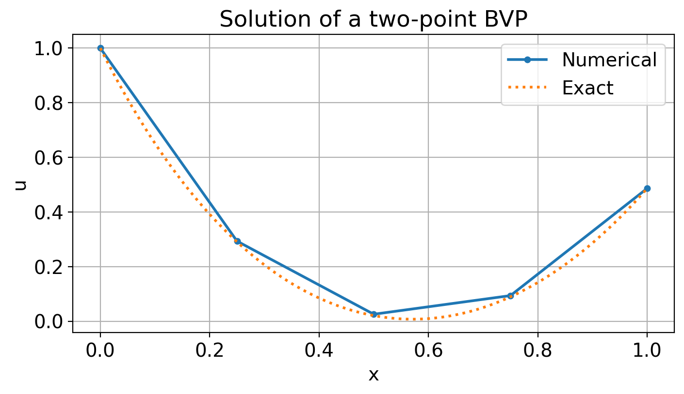
# Plot the solution of the BVP
xe = linspace(0, 1, 101)
plot(x, U, ".-")
plot(xe, u_eksakt(xe), ":")
xlabel("x")
ylabel("u")
legend(["Numerical", "Exact"])
title("Solution of a two-point BVP");

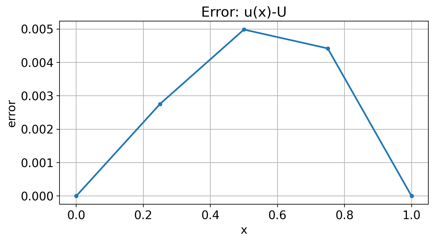
# Plot the error |u(x)-U| in the gridpoints
error = abs(u_eksakt(x) - U)
plot(x, error, ".-")
xlabel("x")
ylabel("error")
title("Error: u(x)-U")
print(f"Max error = {max(abs(error)):.3e}")

Max error = 4.985e-03

56.4. Boundary conditions#

To get a unique solution of a BVP (or a PDE), some information about the solution, usually given on the boundaries has to be known. The most common boundary conditions are:

1. Dirichlet condition: The solution is known at the boundary.

2. Neumann condition: The derivative is known at the boundary.

3. Robin (or mixed) condition: A combination of those.

In the example above, Dirichlet conditions were used. We will now see how to handle Neumann conditions. Robin conditions can be treated similarly.

Given the BVP with a Neumann condition at the left boundary:

Here, $u_a^{\prime }$ is some given value. In this case, the solution $u(a)$ and its corresponding approximation $U_0$ are unknown, and we need some difference formula also for the point $a=x_0$. The simplest option is to use a forward difference

But this is only a first order approximation, and thus lower accuracy is to be expected. We could also use a second order approximation using the values in the grid points $x_0$, $x_1$ and $x_2$, but this will ruin the nice tridiagonal structure of the coefficient matrix.

Instead, use the idea of a false boundary:

Assume that the solution can be stretched outside the boundary $x=a$, all the way to a fictitious grid point $x_{-1}=a-h$, where we also assume there is an approximate and equally fictitious approximation $U_{-1}$ to $u(x_{-1})$. Then we have two difference formulas in the point $a$, one for the BVP itself and a central difference for the boundary conditions:

\begin{align*} \frac{U_{1}-2U_0+U_{-1}}{h^2} + p(x_0)\frac{U_{1}-U_{-1}}{2h} + q(x_0) U_0 & = r(x_0), \ \frac{U_1 - U_{-1}}{2h} &= u’_a. \end{align*}

We can now solve the second equation with respect to $U_{-1}$, and insert the solution into the first equation. This yields the new equation

So the only thing that has changed is the first equation. And since central differences have been used both for the BVP and the boundary condition, the overall order of this approximation can be proved to be 2.

Example 2:

We consider the same example as before, but now with a Neumann condition at the left boundary:

which has the analytic solution $u(x)=e^{-3x}-2e^x-3x-2$.

The modified difference equation at the boundary $x_0=0$ is

We multiply this equation by $h^2$, and include the equation as the discretization for the grid point $x_0$. With this, we obtain the system

\begin{align*} (-2-3h^2)U_0 - 2U_1 &= (2h-2h^2)u’a, \ (1-h)U{i-1} + (-2-3h^2)U_i + (1+h)U_{i+1} &= 9 h^2 x_i, && i=1, \ldots N-1, \ U_N &= u_b, \end{align*}

which, for $N=4$ and $h=0.25$ becomes

The solution of this is

Problem 3:

Now consider the two-point boundary problem from Example 2; that is,

which has the analytic solution $u(x)=e^{-3x}-2e^x-3x-2$.

Here we want you to test the two possible implementations of the Neumann boundary conditions discussed above.

a) Modify the matrix $A$ and right-hand $b$ so that you implement the Neumann boundary condition $u^{\prime }(0)=u_a^{\prime }=-4$ via the approximation $u^{\prime }(a)\approx \frac{U_1-U_0}{h}=u_a^{\prime }$. Now using the analytical solution, run a convergence study a là Problem 2. Plot/write out the resulting EOC table. What convergence order do you get?

b) Now modify the matrix $A$ and right-hand $b$ so that you implement the Neumann boundary condition using the idea of a false boundary as described above. Redo the convergence study, plot/write out the resulting EOC table. What convergence order do you get this time?