48. Polynomial interpolation: Lagrange interpolation#
Anne Kværnø (modified by André Massing)
Date: Jan 13, 2021
If you want to have a nicer theme for your jupyter notebook, download the cascade stylesheet file tma4125.css and execute the next cell:
from math import factorial

import matplotlib.pyplot as plt
import numpy as np
from IPython.core.display import HTML
from numpy import pi
from numpy.linalg import norm, solve  # Solve linear systems and compute norms


def css_styling():
    try:
        with open("tma4125.css") as f:
            styles = f.read()
            return HTML(styles)
    except FileNotFoundError:
        pass  # Do nothing


# Comment out next line and execute this cell to restore the default notebook style
css_styling()
And of course we want to import the required modules.
%matplotlib inline


newparams = {
    "figure.figsize": (6.0, 6.0),
    "axes.grid": True,
    "lines.markersize": 8,
    "lines.linewidth": 2,
    "font.size": 14,
}
plt.rcParams.update(newparams)
49. Introduction#
Polynomials can be used to approximate functions over some bounded interval \(x \in [a,b]\). Such polynomials can be used for different purposes. The function itself may be unknown, and only measured data are available. In this case, a polynomial may be used to find approximations to intermediate values of the function. Polynomials are easy to integrate, and can be used to find approximations of integrals of more complicated functions. This will be exploited later in the course. And there are plenty of other applications.
In this part of the course, we will only discuss interpolation polynomials.
Interpolation problem.
Given \(n+1\) points \((x_i,y_i)_{i=0}^n\). Find a polynomial \(p(x)\) of lowest possible degree satisfying the interpolation condition
The solution \(p(x)\) is called the interpolation polynomial, the \(x_i\) values are called nodes, and the points \((x_i,y_i)\) interpolation points.
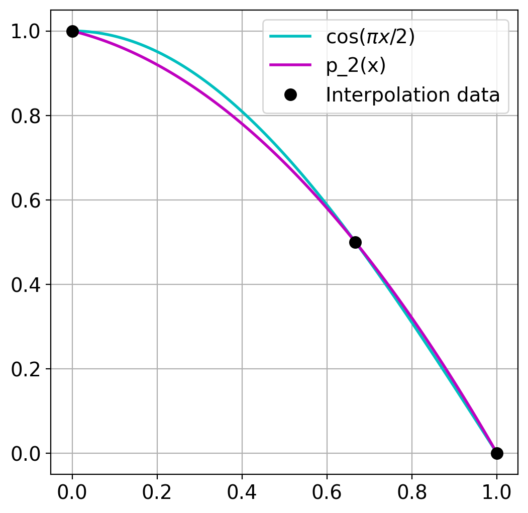
Example 1: Given the points
The corresponding interpolation polynomial is
The \(y\)-values of this example are chosen such that \(y_i=\cos{(\pi x_i/2)}\). So \(p_2(x)\) can be considered as an approximation to \(\cos{(\pi x/2)}\) on the interval \([0,1]\).
# Interpolation data
xdata = [0, 2 / 3.0, 1]
ydata = [1, 1 / 2.0, 0]
# Interpolation polynomial
p2 = lambda x: (-3 * x**2 - x + 4) / 4.0

# Grid points for plotting
x = np.linspace(0, 1, 100)
y = p2(x)

# Original function
f = np.cos(pi * x / 2)

plt.plot(x, f, "c", x, y, "m", xdata, ydata, "ok")
plt.legend([r"$\cos(\pi x/2)$", "p_2(x)", "Interpolation data"])
<matplotlib.legend.Legend at 0x7f84c05a0770>
49.1. Content of this note#
In this part, we will discuss the following:
Method: How to compute the polynomials?
Existence and uniqueness results.
Error analysis: If the polynomial is used to approximate a function, how good is the approximation?
Improvements: If the nodes \(x_i\) can be chosen freely, how should we do it in order to reduce the error?
49.2. Preliminaries#
Let us start with some useful notation and facts about polynomials.
A polynomial of degree \(n\) is given by
\(\mathbb{P}_n\) is the set of all polynomials of degree \(n\).
\(C^m[a,b]\) is the set of all continuous functions that have continuous first \(m\) derivatives.
The value \(r\) is a root or a zero of a polynomial \(p\) if \(p(r)=0\).
A nonzero polynomial of degree \(n\) can never have more than \(n\) real roots (there may be less).
A polynomial of degree \(n\) with \(n\) real roots \(r_1,r_2,\dotsc,r_n\)can be written as
50. Methods#
In this section, we present three techniques for finding the interpolation polynomial for a given set of data.
50.1. The direct approach#
For a polynomial of degree \(n\) the interpolation condition (1) is a linear systems of \(n+1\) equations in \(n+1\) unknowns:
If we are basically interested in the polynomials themself, given by the coefficients \(c_i\), \(i=0,1,\dotsc, n\), this is a perfectly fine solution. It is for instance the strategy implemented in MATLAB’s interpolation routines. However, in this course, polynomial interpolation will be used as a basic tool to construct other algorithms, in particular for integration. In that case, this is not the most convenient option, so we concentrate on a different strategy, which essentially makes it possible to just write up the polynomials.
50.2. Lagrange interpolation#
Given \(n+1\) points \((x_i,y_i)_{i=0}^n\) with distinct \(x_i\) values. The cardinal functions are defined by:
The cardinal functions have the following properties:
\(\ell_i \in \mathbb{P}_n\), \(i=0,1,\dotsc,n\).
\(\ell_i(x_j) = \delta_{ij} = \begin{cases} 1, & \text{when } i=j \\ 0, & \text{when }i\not=j \end{cases}\).
They are constructed solely from the nodes \(x_i\)’s.
They are linearly independent, and thus form a basis for \(\mathbb{P}_{n}\).
Remark. The cardinal functions are also often called Lagrange polynomials.
The interpolation polynomial is now given by
since
Example 2: Given the points:
The corresponding cardinal functions are given by:
and the interpolation polynomial is given by (check it yourself):
50.3. Implementation#
The method above is implemented as two functions:
cardinal(xdata, x): Create a list of cardinal functions \(\ell_i(x)\) evaluated in \(x\).lagrange(ydata, l): Create the interpolation polynomial \(p_n(x)\).
Here, xdata and ydata are arrays with the interpolation points, and x is an
array of values in which the polynomials are evaluated.
You are not required to understand the implementation of these functions, but you should understand how to use them.
newparams = {
    "figure.figsize": (8.0, 4.0),
    "axes.grid": True,
    "lines.markersize": 8,
    "lines.linewidth": 2,
    "font.size": 14,
}
plt.rcParams.update(newparams)
def cardinal(xdata, x):
    """
    cardinal(xdata, x):
    In: xdata, array with the nodes x_i.
        x, array or a scalar of values in which the cardinal functions are evaluated.
    Return: l: a list of arrays of the cardinal functions evaluated in x.
    """
    n = len(xdata)  # Number of evaluation points x
    l = []
    for i in range(n):  # Loop over the cardinal functions
        li = np.ones(len(x))
        for j in range(n):  # Loop to make the product for l_i
            if i is not j:
                li = li * (x - xdata[j]) / (xdata[i] - xdata[j])
        l.append(li)  # Append the array to the list
    return l


def lagrange(ydata, l):
    """
    lagrange(ydata, l):
    In: ydata, array of the y-values of the interpolation points.
         l, a list of the cardinal functions, given by cardinal(xdata, x)
    Return: An array with the interpolation polynomial.
    """
    poly = 0
    for i in range(len(ydata)):
        poly = poly + ydata[i] * l[i]
    return poly
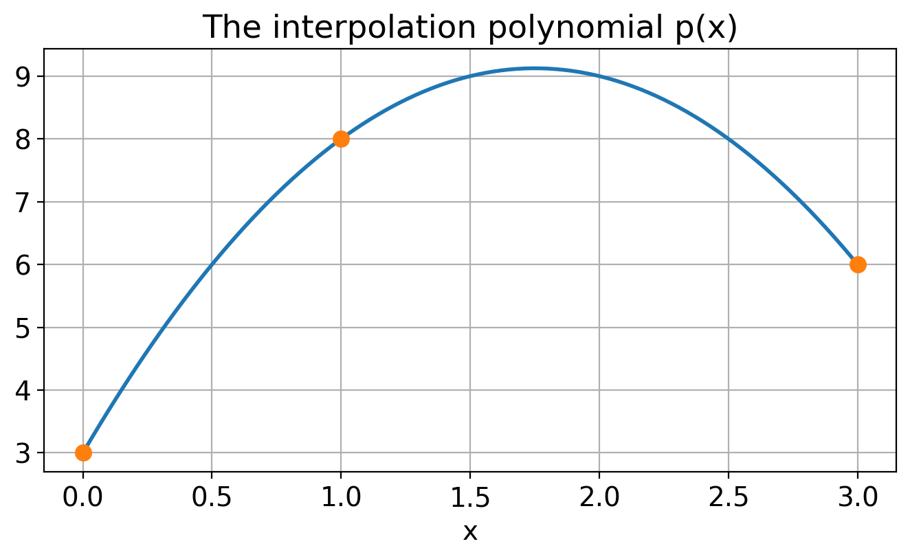
Example 3: Test the functions on the interpolation points of Example 2.
# Example 3
xdata = [0, 1, 3]  # The interpolation points
ydata = [3, 8, 6]
x = np.linspace(0, 3, 101)  # The x-values in which the polynomial is evaluated
l = cardinal(xdata, x)  # Find the cardinal functions evaluated in x
p = lagrange(ydata, l)  # Compute the polynomial evaluated in x
plt.plot(x, p)  # Plot the polynomial
plt.plot(xdata, ydata, "o")  # Plot the interpolation points
plt.title("The interpolation polynomial p(x)")
plt.xlabel("x");
Numerical exercises:
Plot the cardinal functions for the nodes of Example 1.
Plot the interpolation polynomials for some points of your own choice.
# Insert your code here (use "+" in the Toolbar menu for more cells)
50.4. Existence and uniqueness of interpolation polynomials.#
We have already proved the existence of such polynomials, simply by constructing them. But are they unique? The answer is yes!
Theorem: Existence and uniqueness.
Given \(n+1\) points \((x_i,y_i)_{i=0}^n\) with distinct \(x\) values. Then there is one and only one polynomial \(p_n(x) \in \mathbb{P}_n\) satisfying the interpolation condition
Proof. Suppose there exist two different interpolation polynomials \(p_n\) and \(q_n\) of degree \(n\) interpolating the same \(n+1\) points. The polynomial \(r(x) = p_n(x)-q_n(x)\) is of degree \(n\) with zeros in all the nodes \(x_i\), that is a total of \(n+1\) zeros. But then \(r\equiv 0\), and the two polynomials \(p_n\) and \(q_n\) are identical.