44. The Spectral Element Method - Numerical Integration - The Gauss-Lobatto-Legendre approach#
The following notebook presents a basic integration scheme that we’re going to use in the Spectral Element Code to calculate the entries of the mass and stiffness matrices.
Fundamental principal:
Replace the function \(f(x)\) that we want to integrate by a polynomial approximation that can be integrated analytically.
As interpolating functions we use the Lagrange polynomials \(l_i\) and obtain the following integration scheme for an arbitrary function \(f(x)\) defined on the interval \([-1,1]\) : \begin{eqnarray*} \int_{-1}^1 f(x) \ dx \approx \int {-1}^1 P_N(x) dx = \sum{i=1}^{N+1} w_i f(x_i) \end{eqnarray*} with \begin{eqnarray*} P_N(x)= \sum_{i=1}^{N+1} f(x_i) \ l_i^{(N)}(x). \end{eqnarray*} As collocation points we use the Gauss-Lobatto-Legendre points \(x_i\) and the corresponding weights that are needed to evaluate the integral are calculated as follows: \begin{eqnarray*} w_i= \int_{-1}^1 l_i^{(N)}(x) \ dx \end{eqnarray*}.
We want to investigate the performance of
the numerical integration scheme. You can use the gll() routine to
obtain the differentiation weights \(w_i\) for an
arbitrary function f(x) and the relevant integration points \(x_i\).
44.1. 1. Numerical integration of an arbritrary function:#
Define a function \(f(x)\) of your choice and calculate analytically the integral \(\int f(x) \ dx\) for the interval \([−1, 1]\). Perform the integration numerically and compare the results.
44.2. 2. The order of integration#
Take a closer look and modify the function and the order of the numerical integration.
import matplotlib.pyplot as plt
import numpy as np
from gll import gll
from lagrange2 import lagrange2
# Show Plot in The Notebook
# matplotlib.use("nbagg")
# Prettier plots.
plt.style.use("ggplot")
# Exercise for Gauss integration
n = 1000
x = np.linspace(-1, 1, n)
# MODIFY f and intf to test different functions!
# f = np.sin(x * np.pi)
f = x + x * x + np.sin(x)
# Analytical value of the DEFINITE integral from -1 to 1
# intf = 1.0 / np.pi * (-np.cos(1.0 * np.pi) + np.cos(-1.0 * np.pi))
intf = 2.0 / 3.0
# Choose order
N = 6
# Get integration points and weights from the gll routine
xi, w = gll(N)
# Initialize function at points xi
fi = np.interp(xi, x, f)
################################################
# Evaluate integral
intfn = 0
for i in range(len(w)):
intfn = intfn + w[i] * fi[i]
################################################
# Calculate Lagrange Interpolant for plotting purposes.
lp = np.zeros((N + 1, len(x)))
for i in range(0, len(x)):
for j in range(-1, N):
lp[j + 1, i] = lagrange2(N, j, x[i], xi)
s = np.zeros_like(x)
for j in range(0, N + 1):
s = s + lp[j, :] * fi[j]
print("Solution of the analytical integral: %g" % intf)
print("Solution of the numerical integral: %g" % intfn)
# -------------------
# Plot results
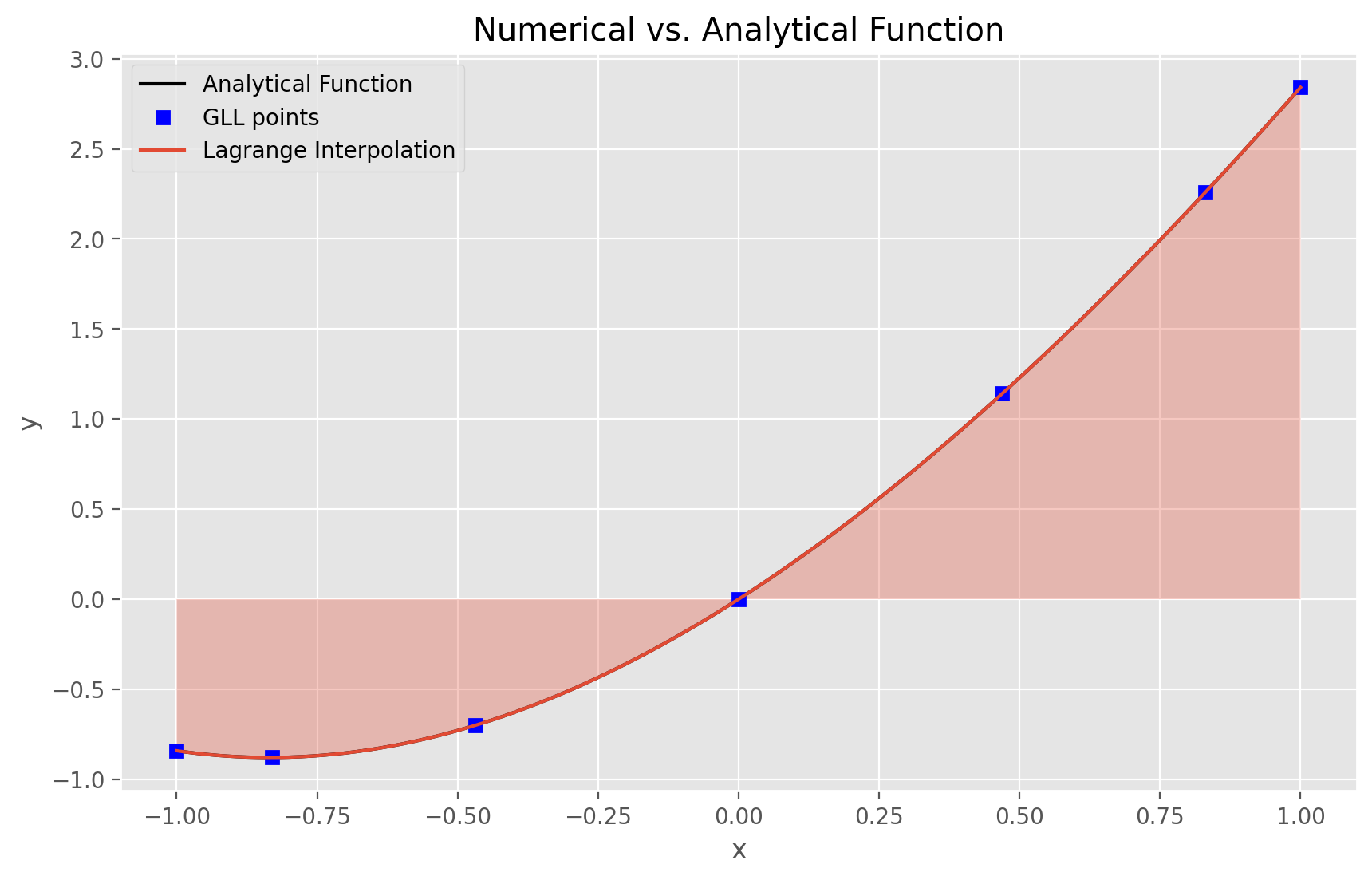
plt.figure(figsize=(10, 6))
plt.plot(x, f, "k-", label="Analytical Function")
plt.plot(xi, fi, "bs", label="GLL points")
plt.plot(x, s, label="Lagrange Interpolation")
plt.fill_between(x, s, np.zeros_like(x), alpha=0.3)
plt.xlabel("x")
plt.ylabel("y")
plt.title("Numerical vs. Analytical Function")
plt.legend()
plt.show()
Solution of the analytical integral: 0.666667
Solution of the numerical integral: 0.666668