Acoustic Waves 2D - Heterogeneous case

33. Acoustic Waves 2D - Heterogeneous case#

This exercise covers the following aspects:

Presenting you with an implementation of the 2D acoustic wave equation
Allowing you to explore the benefits of using high-order finite-difference operators
Understanding the concepts of stability (Courant criterion)
Exploration of numerical dispersion and numerical grid anisotropy
Changing the earth model and exploring some effects of structural heterogeneities (e.g., fault zones)

33.1. Basic Equations#

The acoustic wave equation in 2D is $ $\ddot{p} (x, z, t) = c (x, z)^{2} (\partial_{x}^{2} p (x, z, t) + \partial_{z}^{2} p (x, z, t)) + s (x, z, t)$ $

and we replace the time-dependent (upper index time, lower indices space) part by

\frac{p_{j, k}^{n + 1} - 2 p_{j, k}^{n} + p_{j, k}^{n - 1}}{d t^{2}} = c_{j}^{2} (\partial_{x}^{2} p + \partial_{z}^{2} p) + s_{j, k}^{n}

solving for $p_{j, k}^{n + 1}$ . The extrapolation scheme is $$ p_{j,k}^{n+1} \ = \ c_j^2 \mathrm{d}t^2 \left[ \partial_x^2 p + \partial_z^2 p \right]

2p_{j,k}^n - p_{j,k}^{n-1} + \mathrm{d}t^2 s_{j,k}^n $$ The space derivatives are determined by

\partial_{x}^{2} p = \frac{p_{j + 1, k}^{n} - 2 p_{j, k}^{n} + p_{j - 1, k}^{n}}{d x^{2}}

\partial_{z}^{2} p = \frac{p_{j, k + 1}^{n} - 2 p_{j, k}^{n} + p_{j, k - 1}^{n}}{d z^{2}}

33.1.1. 1. Getting started#

Relate the time extrapolation loop with the numerical algorithm we developed in the course. Understand the input parameters for the simulation and the plots that are generated. Modify source and receiver locations and observe the effects on the seismograms.

33.1.2. 2. Stability#

The Courant criterion is defined as $e p s = (v \cdot d t) / d x$ and provides the maximum possible, stable time step, with $v$ beeing the velocity, $d t$ the time step and $d x$ the spatial step. Determine numerically the stability limit of the code as accurately as possible by increasing the time step. Print the max value of the pressure field at each time step and observe the evolution of it in the case of stable and unstable simulations.

33.1.3. 3. High-order operators#

Extend the code by adding the option to use a 5-point difference operator. Compare simulations with the 3-point and 5-point operator. Is the stability limit still the same? Estimate the number of points per wavelength and investigate the accuracy of the simulation by looking for signs of numerical dispersion in the resulting seismograms. The 5-pt weights are: $[- 1 / 12, 4 / 3, - 5 / 2, 4 / 3, - 1 / 12] / d x^{2}$ .

33.1.4. 4. Numerical anisotropy#

Increase the frequency of the wavefield by varying $f_{0}$ . Investigate the angular dependence of the wavefield. Why does the wavefield look anisotropic? Which direction is the most accurate and why? What happens if you set the source time function to a spike (zero everywhere except one element with value $1$ ).

33.1.5. 5. Heterogeneous models#

Now let us explore the power of the finite-difference method by varying the internal structure of the model. Here we can only modify the velocity $c$ that can vary at each grid point (any restrictions?). Here are some suggestions: investigate the influence of the structure by analysing the snapshots and the seismograms.

Add a low(high) velocity layer near the surface. Put the source at $z_{s} = 2$ .
Add a vertical low velocity zone (fault zone) of a certain width (e.g. $10$ grid points), and discuss the resulting wavefield
Simulate topography by setting the pressure to $0$ above the surface. Use a Gaussian hill shape or a random topography.
etc.

33.1.6. 6. Source-receiver reciprocity#

Initialize a strongly heterogeneous 2D velocity model of your choice and simulate waves propagating from an internal source point ( $x_{s}, z_{s}$ ) to an internal receiver ( $x_{r}, z_{r}$ ). Show that by reversing source and receiver you obtain the same seismogram.

33.1.7. 7. Time reversal#

Time reversal. Define in an arbitrary 2D velocity model a source at the centre of the domain an a receiver circle at an appropriate distance around the source. Simulate a wavefield, record it at the receiver ring and store the results. Reverse the synthetic seismograms and inject the as sources at the receiver points. What happens? Do you know examples where this principle is used?

# This is a configuration step for the exercise. Please run it before the simulation code!
import matplotlib.pyplot as plt
import numpy as np

Below is the 2D acoustic simulation code:

# Simple finite difference solver
# Acoustic wave equation  p_tt = c^2 p_xx + src
# 2-D regular grid

nx = 200  # grid points in x - 500
nz = 200  # grid points in z - 500
nt = 1000  # number of time steps
dx = 10.0  # grid increment in x - 1
dt = 0.001  # Time step
c0 = 3000.0  # velocity (can be an array) - 580
isx = nx // 2  # source index x - 250
isz = nz // 2  # source index z - 250
ist = 100  # shifting of source time function
f0 = 50.0  # dominant frequency of source (Hz)
isnap = 10  # snapshot frequency
T = 1.0 / f0  # dominant period
nop = 5  # length of operator

# Model type, available are "homogeneous", "fault_zone",
# "surface_low_velocity_zone", "random", "topography",
# "slab"
model_type = "fault_zone"

# Receiver locations
irx = np.array([60, 80, 100, 120, 140])
irz = np.array([5, 5, 5, 5, 5])
seis = np.zeros((len(irx), nt))

# Initialize pressure at different time steps and the second
# derivatives in each direction
p = np.zeros((nz, nx))
pold = np.zeros((nz, nx))
pnew = np.zeros((nz, nx))
pxx = np.zeros((nz, nx))
pzz = np.zeros((nz, nx))

# Initialize velocity model (the fun bit!)
c = np.zeros((nz, nx))

if model_type == "homogeneous":
    c += c0
elif model_type == "fault_zone":
    c += c0
    c[:, nx // 2 - 5 : nx // 2 + 5] *= 0.8
elif model_type == "surface_low_velocity_zone":
    c += c0
    c[1:10, :] *= 0.8
elif model_type == "random":
    pert = 0.4
    r = 2.0 * (np.random.rand(nz, nx) - 0.5) * pert
    c += c0 * (1 + r)
elif model_type == "topography":
    c += c0
    c[0:10, 10:50] = 0
    c[0:10, 105:115] = 0
    c[0:30, 145:170] = 0
    c[10:40, 20:40] = 0
    c[0:15, 50:105] *= 0.8
elif model_type == "slab":
    c += c0
    c[110:125, 0:125] = 1.4 * c0
    for i in range(110, 180):
        c[i, i - 5 : i + 15] = 1.4 * c0
else:
    raise NotImplementedError

cmax = c.max()

# Source time function Gaussian, nt + 1 as we loose the last one by diff
src = np.empty(nt + 1)
for it in range(nt):
    src[it] = np.exp(-1.0 / T**2 * ((it - ist) * dt) ** 2)
# Take the first derivative
src = np.diff(src) / dt
src[nt - 1] = 0

# Plot preparation

v = max([np.abs(src.min()), np.abs(src.max())])
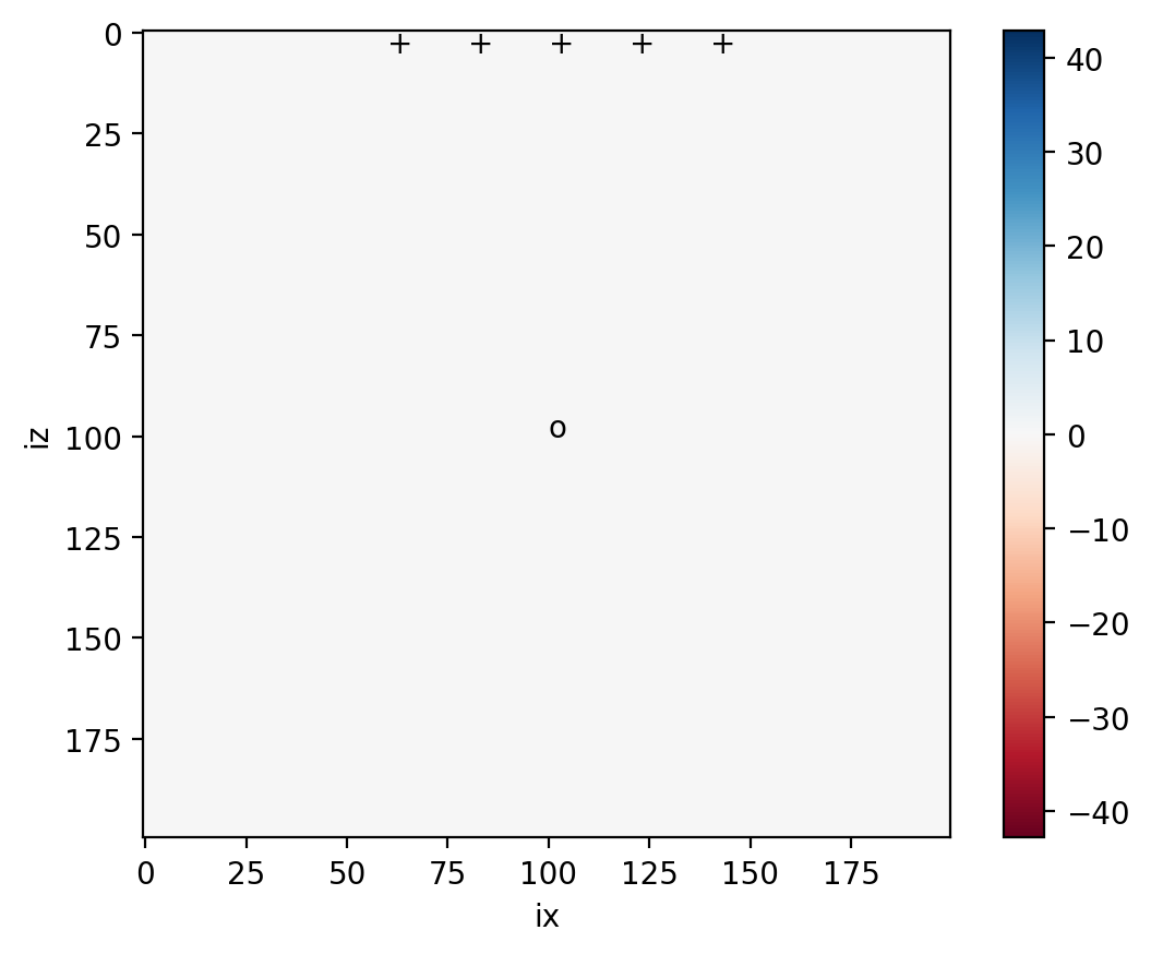
# Initialize animated plot
image = plt.imshow(
    pnew, interpolation="nearest", animated=True, vmin=-v, vmax=+v, cmap=plt.cm.RdBu
)


# Plot the receivers
for x, z in zip(irx, irz):
    plt.text(x, z, "+")

plt.text(isx, isz, "o")
plt.colorbar()
plt.xlabel("ix")
plt.ylabel("iz")


plt.ion()
# plt.show(block=False)

# required for seismograms
ir = np.arange(len(irx))

# Output Courant criterion
print("Courant Criterion eps :")
print(cmax * dt / dx)

Courant Criterion eps :
0.3

../_images/a3a9306f7914f42848c23a03935426493b4f0d1f97683a980e711bb5732af895.png

# Time extrapolation
for it in range(nt):
    if nop == 3:
        # calculate partial derivatives, be careful around the boundaries
        for i in range(1, nx - 1):
            pzz[:, i] = p[:, i + 1] - 2 * p[:, i] + p[:, i - 1]
        for j in range(1, nz - 1):
            pxx[j, :] = p[j - 1, :] - 2 * p[j, :] + p[j + 1, :]

    if nop == 5:
        # calculate partial derivatives, be careful around the boundaries
        for i in range(2, nx - 2):
            pzz[:, i] = (
                -1.0 / 12 * p[:, i + 2]
                + 4.0 / 3 * p[:, i + 1]
                - 5.0 / 2 * p[:, i]
                + 4.0 / 3 * p[:, i - 1]
                - 1.0 / 12 * p[:, i - 2]
            )
        for j in range(2, nz - 2):
            pxx[j, :] = (
                -1.0 / 12 * p[j + 2, :]
                + 4.0 / 3 * p[j + 1, :]
                - 5.0 / 2 * p[j, :]
                + 4.0 / 3 * p[j - 1, :]
                - 1.0 / 12 * p[j - 2, :]
            )

    pxx /= dx**2
    pzz /= dx**2

    # Time extrapolation
    pnew = 2 * p - pold + dt**2 * c**2 * (pxx + pzz)
    # Add source term at isx, isz
    pnew[isz, isx] = pnew[isz, isx] + src[it]

    # Plot every isnap-th iteration
    if (
        it % isnap == 0
    ):  # you can change the speed of the plot by increasing the plotting interval
        plt.title("Max P: %.2f" % p.max())
        image.set_data(pnew)
        plt.gcf().canvas.draw()

    pold, p = p, pnew

    # Save seismograms
    seis[ir, it] = p[irz[ir], irx[ir]]

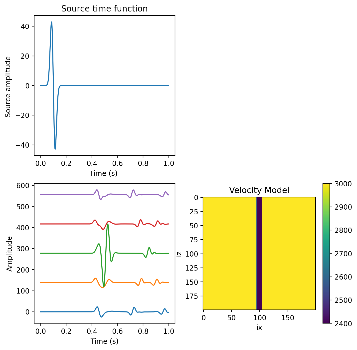
../_images/19b627fe64f8c892ce7e32c9d07aedb144a1bc96f3dcb5c82e791128ca6c750a.png

The cell below allows you to plot source time function, seismic velocites, and the resulting seismograms in windows inside the notebook. Remember to rerun after you simulated again!

# Plot the source time function and the seismograms

plt.ioff()
plt.figure(figsize=(8, 8))

plt.subplot(221)
time = np.arange(nt) * dt
plt.plot(time, src)
plt.title("Source time function")
plt.xlabel("Time (s) ")
plt.ylabel("Source amplitude ")

# plt.subplot(222)
# ymax = seis.ravel().max()
# for ir in range(len(seis)):
#    plt.plot(time, seis[ir, :] + ymax * ir)
#    plt.xlabel('Time (s)')
#    plt.ylabel('Amplitude')

plt.subplot(223)
ymax = seis.ravel().max()
for ir in range(len(seis)):
    plt.plot(time, seis[ir, :] + ymax * ir)
    plt.xlabel("Time (s)")
    plt.ylabel("Amplitude")

plt.subplot(224)
# The velocity model is influenced by the Earth model above
plt.title("Velocity Model")
plt.imshow(c)
plt.xlabel("ix")
plt.ylabel("iz")
plt.colorbar()
plt.show()

../_images/75845ab2e2f1c203226fa631a9cf987dbba3f2893c9eec4ba906e442fb41e628.png