Acoustic Waves 1D I

30. Acoustic Waves 1D I#

This notebook covers the following aspects:

Implementation of the 1D acoustic wave equation
Understanding the input parameters for the simulation and the plots that are generated
Understanding the concepts of stability (Courant criterion)
Modifying source and receiver locations and observing the effects on the seismograms

30.1. Exercises:#

Check out the FD algorithm in the last cell
Modify the frequency of the source wave let (e.g. in the interval 10 to 100 Hz) and observe how the solution accuracy changes
Increase the time step dt and observe what happens (at some point the solution gets unstable).

Note: Corrections May 14, 2020

Error in the source time function and filter calculation corrected
Exercises added

30.2. Numerical Solution (Finite Differences Method)#

The acoustic wave equation in 1D with constant density

\partial_{t}^{2} p (x, t) = {(c (x))}^{2} \partial_{x}^{2} p (x, t) + s (x, t)

with pressure $p$ , acoustic velocity $c$ , and source term $s$ contains two second derivatives that can be approximated with a difference formula such as

\partial_{t}^{2} p (x, t) \approx \frac{p (x, t + d t) - 2 p (x, t) + p (x, t - d t)}{d t^{2}}

and equivalently for the space derivative. Injecting these approximations into the wave equation allows us to formulate the pressure p(x) for the time step $t + d t$ (the future) as a function of the pressure at time $t$ (now) and $t - d t$ (the past). This is called an explicit scheme allowing the extrapolation of the space-dependent field into the future only looking at the nearest neighbourhood.

We replace the time-dependent (upper index time, lower indices space) part by

\[ \frac{p_{i}^{n+1}-2p_{i}^{n}+p_{i}^{n-1}}{\left(\mathrm{d}t\right)^{2]}= c^{2}\left(\partial_x^2 p\right)+ s_{i}^{n} \]

solving for $p_{i}^{n + 1}$ .

The extrapolation scheme is

p_{i}^{n + 1} = c_{i}^{2} {(d t)}^{2} [\partial_{x}^{2} p] + 2 p_{i}^{n} - p_{i}^{n - 1} + {(d t)}^{2} s_{i}^{n}

The space derivatives are determined by

\partial_{x}^{2} p = \frac{p_{i + 1}^{n} - 2 p_{i}^{n} + p_{i - 1}^{n}}{{(d x)}^{2}}

import warnings

import matplotlib
import matplotlib.pyplot as plt
import numpy as np
from matplotlib import gridspec, use

# matplotlib.use("nbagg")
warnings.filterwarnings("ignore")

# Parameter Configuration
# -----------------------

nx = 10000  # number of grid points in x-direction
xmax = 10000  # physical domain (m)
dx = xmax / (nx - 1)  # grid point distance in x-direction
c0 = 334.0  # wave speed in medium (m/s)
isrc = int(nx / 2)  # source location in grid in x-direction
# ir   = isrc + 100          # receiver location in grid in x-direction
nt = 1001  # maximum number of time steps
dt = 0.0010  # time step

# Source time function parameters
f0 = 25.0  # dominant frequency of the source (Hz)
t0 = 4.0 / f0  # source time shift

# Snapshot
idisp = 5  # display frequency

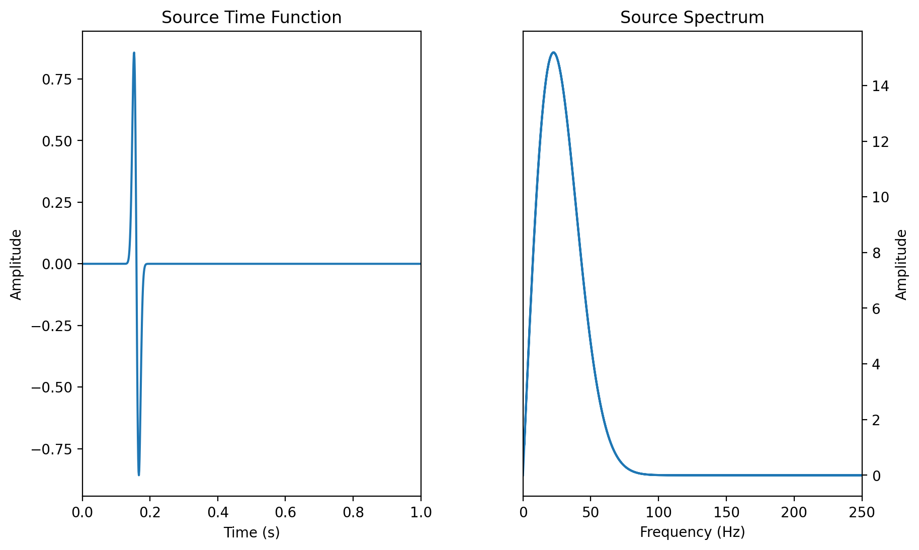
# Plot Source Time Function
# -------------------------

# Source time function (Gaussian)
# -------------------------------
src = np.zeros(nt + 1)
time = np.linspace(0 * dt, nt * dt, nt)
# 1st derivative of a Gaussian
src = -8.0 * (time - t0) * f0 * (np.exp(-1.0 * (4 * f0) ** 2 * (time - t0) ** 2))

# Plot source time function

# Plot position configuration
# ---------------------------
plt.ion()
fig1 = plt.figure(figsize=(10, 6))
gs1 = gridspec.GridSpec(1, 2, width_ratios=[1, 1], hspace=0.3, wspace=0.3)

# Plot source time function
# -------------------------
ax1 = plt.subplot(gs1[0])
ax1.plot(time, src)  # plot source time function
ax1.set_title("Source Time Function")
ax1.set_xlim(time[0], time[-1])
ax1.set_xlabel("Time (s)")
ax1.set_ylabel("Amplitude")

# Plot source spectrum
# --------------------
ax2 = plt.subplot(gs1[1])
spec = np.fft.fft(src)  # source time function in frequency domain
freq = np.fft.fftfreq(spec.size, d=dt)  # time domain to frequency domain
ax2.plot(np.abs(freq), np.abs(spec))  # plot frequency and amplitude
ax2.set_xlim(0, 250)  # only display frequency from 0 to 250 Hz
ax2.set_title("Source Spectrum")
ax2.set_xlabel("Frequency (Hz)")
ax2.set_ylabel("Amplitude")
ax2.yaxis.tick_right()
ax2.yaxis.set_label_position("right")

../_images/2de9fc95fddd89dc6468a9f79e3e74cd1939303ebc39858843ce760848bc375c.png

# Plot Snapshot & Seismogram
# ---------------------------------------------------------------------------

# Initialize empty pressure
# -------------------------
p = np.zeros(nx)  # p at time n (now)
pold = np.zeros(nx)  # p at time n-1 (past)
pnew = np.zeros(nx)  # p at time n+1 (present)
d2px = np.zeros(nx)  # 2nd space derivative of p

# Initialize model (assume homogeneous model)
# -------------------------------------------
c = np.zeros(nx)
c = c + c0  # initialize wave velocity in model

# Initialize coordinate
# ---------------------
x = np.arange(nx)
x = x * dx  # coordinate in x-direction


# Plot position configuration
# ---------------------------
plt.ion()
fig2 = plt.figure(figsize=(10, 6))
gs2 = gridspec.GridSpec(1, 1, width_ratios=[1], hspace=0.3, wspace=0.3)

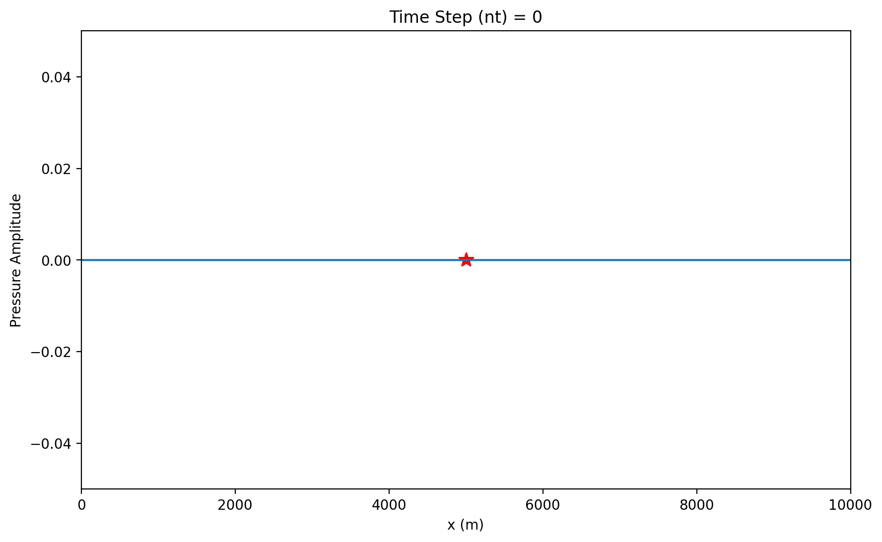
# Plot 1D wave propagation
# ------------------------
# Note: comma is needed to update the variable
ax3 = plt.subplot(gs2[0])
(leg1,) = ax3.plot(
    isrc, 0, "r*", markersize=11
)  # plot position of the source in snapshot
# leg2,= ax3.plot(ir, 0, 'k^', markersize=8) # plot position of the receiver in snapshot
(up31,) = ax3.plot(p)  # plot pressure update each time step
ax3.set_xlim(0, xmax)
ax3.set_ylim(-np.max(p), np.max(p))
ax3.set_title("Time Step (nt) = 0")
ax3.set_xlabel("x (m)")
ax3.set_ylabel("Pressure Amplitude");
# ax3.legend((leg1, leg2), ('Source', 'Receiver'), loc='upper right', fontsize=10, numpoints=1)

../_images/ceed866e459e3d9f19dca953f13236a9cac57886c9e41c1695842da67d2e369f.png

# 1D Wave Propagation (Finite Difference Solution)
# ------------------------------------------------

# Loop over time
for it in range(nt):
    # 2nd derivative in space
    for i in range(1, nx - 1):
        d2px[i] = (p[i + 1] - 2 * p[i] + p[i - 1]) / dx**2

    # Time Extrapolation
    # ------------------
    pnew = 2 * p - pold + c**2 * dt**2 * d2px

    # Add Source Term at isrc
    # -----------------------
    # Absolute pressure w.r.t analytical solution
    pnew[isrc] = pnew[isrc] + src[it] / (dx) * dt**2

    # Remap Time Levels
    # -----------------
    pold, p = p, pnew

    # Plot pressure field
    # -------------------------------------
    if (it % idisp) == 0:
        ax3.set_title("Time Step (nt) = %d" % it)
        ax3.set_ylim(-1.1 * np.max(abs(p)), 1.1 * np.max(abs(p)))
        # plot around propagating wave
        window = 100
        xshift = 25
        ax3.set_xlim(
            isrc * dx + c0 * it * dt - window * dx - xshift,
            isrc * dx + c0 * it * dt + window * dx - xshift,
        )
        up31.set_ydata(p)
        plt.gcf().canvas.draw()

<Figure size 640x480 with 0 Axes>

Acoustic Waves 1D I

Contents

30. Acoustic Waves 1D I#

30.1. Exercises:#

30.2. Numerical Solution (Finite Differences Method)#