Computers, Waves, Simulations

The Pseudo-Spectral Method - Elastic Wave Equation 1D

38. The Pseudo-Spectral Method - Elastic Wave Equation 1D

This notebook covers the following aspects:

• Initialize the Chebyshev derivative matrix \(D_{ij}\) and display the Chebyshev derivative matrix

• Define and initialize space, material and source parameters

• Extrapolate time using the previously defined Chebyshev derivative matrix

Update May 13, 2020

• Change naming of fields from p to u to make it compatible with equations

• Added option for mu and ro to be heterogeneous (i.e., now defined as vectors)

• Made space derivative calculations consistent with elastic equation

38.1. Basic Equations

This notebook presents the numerical solution for the 1D elastic wave equation using the Chebyshev Pseudospectral Method. We depart from the equation

\begin{equation} \rho(x) \partial_t^2 u(x,t) = \partial_x (\mu(x) \partial_x u(x,t)) + f(x,t), \end{equation}

and use a standard 3-point finite-difference operator to approximate the time derivatives. Then, the displacement field is extrapolated as

\begin{equation} \rho_i\frac{u_{i}^{j+1} - 2u_{i}^{j} + u_{i}^{j-1}}{dt^2}= \partial_x (\mu(x) \partial_x u(x,t)){i}^{j} + f{i}^{j} \end{equation}

An alternative way of performing space derivatives of a function defined on the Chebyshev collocation points is to define a derivative matrix \(D_{ij}\)

\begin{equation} D_{ij} = \begin{cases} -\frac{2 N^2 + 1}{6} \hspace{1.5cm} \text{for i = j = N}\ -\frac{1}{2} \frac{x_i}{1-x_i^2} \hspace{1.5cm} \text{for i = j = 1,2,…,N-1}\ \frac{c_i}{c_j} \frac{(-1)^{i+j}}{x_i - x_j} \hspace{1.5cm} \text{for i \(\neq\) j = 0,1,…,N} \end{cases} \end{equation}

where \(N+1\) is the number of Chebyshev collocation points \( \ x_i = cos(i\pi / N)\), \( \ i=0,...,N\) and the \(c_i\) are given as

\[ c_i = 2 \hspace{1.5cm} \text{for i = 0 or N} \]

\[ c_i = 1 \hspace{1.5cm} \text{otherwise} \]

This differentiation matrix allows us to write the derivative of the function \(f_i = f(x_i)\) (possibly depending on time) simply as

\[\partial_x u_i = D_{ij} \ u_j\]

where the right-hand side is a matrix-vector product, and the Einstein summation convention applies.

import warnings

import matplotlib
import matplotlib.pyplot as plt
import numpy as np
from matplotlib import gridspec, use

# Import python function from the file "ricker.py"
from ricker import ricker

# matplotlib.use("nbagg")
warnings.filterwarnings("ignore")

38.1.1. 1. Chebyshev derivative method

# Define Function that initializes the Chebyshev derivative matrix D_{ij}


def get_cheby_matrix(nx):
    cx = np.zeros(nx + 1)
    x = np.zeros(nx + 1)
    for ix in range(0, nx + 1):
        x[ix] = np.cos(np.pi * ix / nx)

    cx[0] = 2.0
    cx[nx] = 2.0
    cx[1:nx] = 1.0

    D = np.zeros((nx + 1, nx + 1))
    for i in range(0, nx + 1):
        for j in range(0, nx + 1):
            if i == j and i != 0 and i != nx:
                D[i, i] = -x[i] / (2.0 * (1.0 - x[i] * x[i]))
            else:
                D[i, j] = (cx[i] * (-1) ** (i + j)) / (cx[j] * (x[i] - x[j]))

    D[0, 0] = (2.0 * nx**2 + 1.0) / 6.0
    D[nx, nx] = -D[0, 0]
    return D


# Call the chebyshev differentiation matrix
# ---------------------------------------------------------------
D_ij = get_cheby_matrix(50)

# ---------------------------------------------------------------
# Display Differentiation Matrix
# ---------------------------------------------------------------
plt.imshow(D_ij, interpolation="bicubic", cmap="gray")
plt.title("Differentiation Matrix $D_{ij}$")
plt.axis("off")
plt.tight_layout()

38.1.2. 2. Initialization of setup

# Basic parameters
# ---------------------------------------------------------------
tmax = 0.0003  # Seismogram length
eps = 1.4  # stability limit
isx = 100  # Index of source location
lw = 0.7  # Linewidth
f0 = 50000  # dominant frequency
iplot = 20  # Snapshot frequency

# space domain
nx = 100  # number of grid points in x 199
xs = np.floor(nx / 2)  # source location
x = np.zeros(nx + 1)

# initialization of pressure fields
u = np.zeros(nx + 1)
unew = np.zeros(nx + 1)
uold = np.zeros(nx + 1)
d2u = np.zeros(nx + 1)

# Background elastic parameters
rho0 = 2500.0  # kg/m^3
c0 = 3000.0  # m/s
mu0 = rho0 * c0**2  # Pa

# material parameters (in vector)
rho = np.zeros(nx + 1) + rho0
c = np.zeros(nx + 1) + c0
mu = np.zeros(nx + 1) + mu0


# material parameters (heterogeneous case, uncomment if desired)
# mu[:np.int(nx/3)]  = 0.6*mu[:np.int(nx/3)]
# c = np.sqrt(mu/rho)

# Initialize spatial domain [-1, 1]
for ix in range(0, nx + 1):
    x[ix] = np.cos(ix * np.pi / nx)
dxmin = min(abs(np.diff(x)))
dxmax = max(abs(np.diff(x)))

dt = eps * dxmin / np.max(c)  # calculate time step from stability criterion
nt = int(round(tmax / dt))  # Number of time steps

38.1.3. 3. Source Initialization

# source time function
# ---------------------------------------------------------------
t = np.arange(1, nt + 1) * dt  # initialize time axis
T0 = 1.0 / f0
tmp = ricker(dt, T0)
isrc = tmp
tmp = np.diff(tmp)
src = np.zeros(nt)
src[0 : np.size(tmp)] = tmp

# spatial source function
# ---------------------------------------------------------------
sigma = 1.5 * dxmax
x0 = x[int(xs)]
sg = np.exp(-1 / sigma**2 * (x - x0) ** 2)
sg = sg / max(sg)

38.1.4. 4. Time Extrapolation

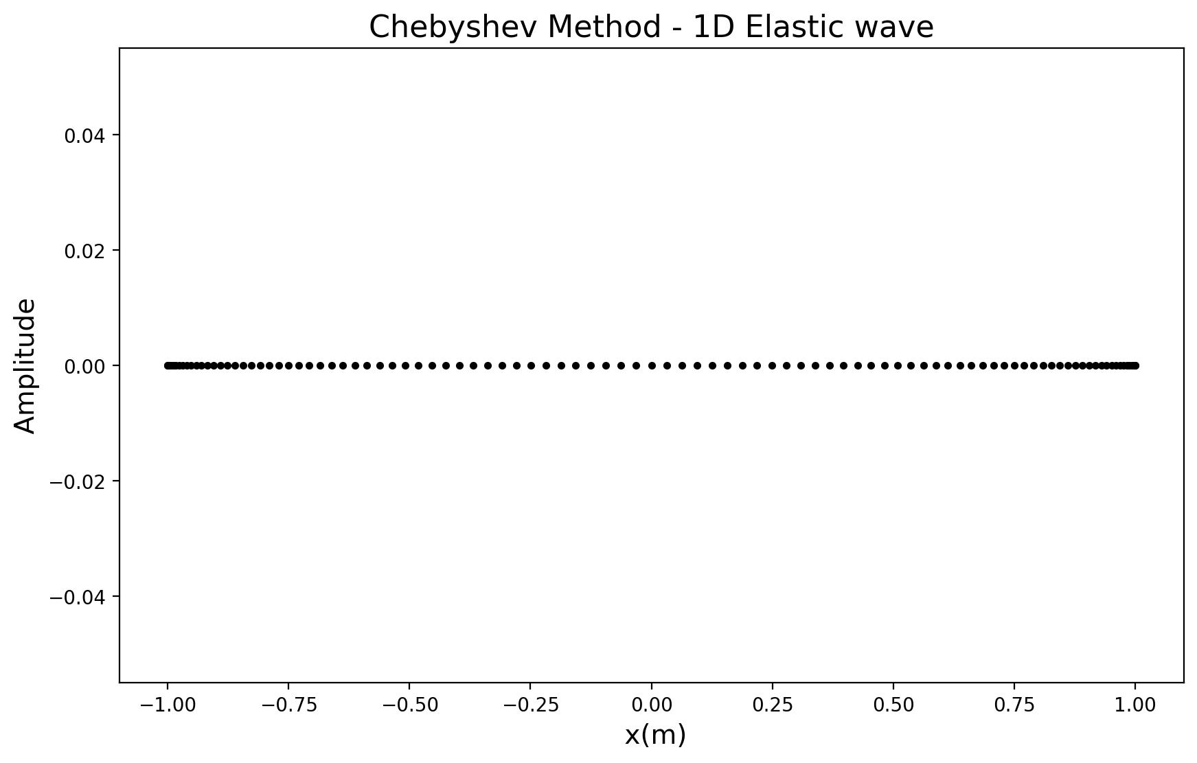
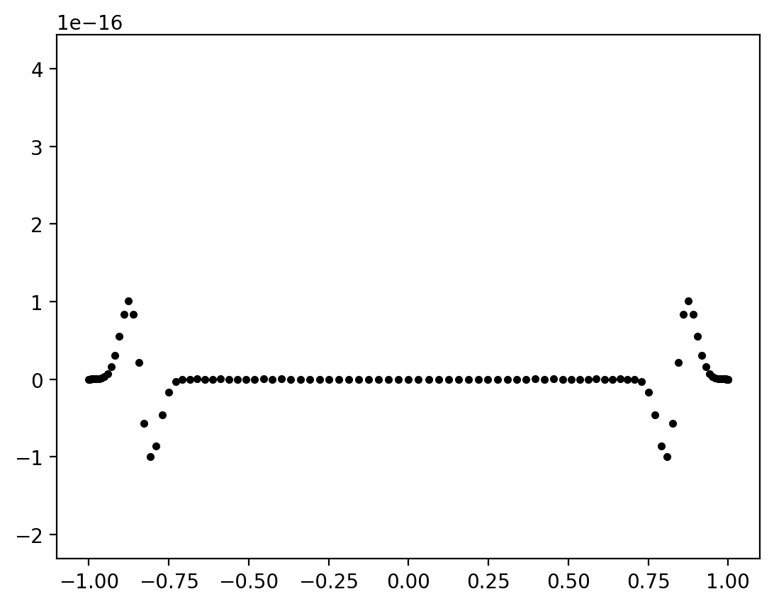
Now we time extrapolate using the previously defined get_cheby_matrix(nx) method to call the differentiation matrix. The discrete values of the numerical simulation are indicated by dots in the animation, they represent the Chebyshev collocation points. Observe how the wavefield near the domain center is less dense than towards the boundaries.

Note: The wavefield is plotted with dots in order to indicate the densification of the grid near the boundaries and the small number of points per wavelength required.

# Initialize animated plot
# ---------------------------------------------------------------
plt.figure(figsize=(10, 6))
line = plt.plot(x, u, "k.", lw=2)
plt.title("Chebyshev Method - 1D Elastic wave", size=16)
plt.xlabel(" x(m)", size=14)
plt.ylabel(" Amplitude ", size=14)

plt.ion()  # set interactive mode
plt.show()
# ---------------------------------------------------------------
# Time extrapolation
# ---------------------------------------------------------------
# Differentiation matrix
D = get_cheby_matrix(nx)
for it in range(nt):
    # Space derivatives (corrected May 11, 2020)
    du = mu * D @ u
    du = D @ du / rho

    # Time extrapolation
    unew = 2 * u - uold + np.transpose(du) * dt**2

    # Source injection
    unew = unew + sg * src[it] * dt**2 / rho

    # Remapping
    uold, u = u, unew
    u[0] = 0
    u[nx] = 0  # set boundaries pressure free

    # --------------------------------------
    # Animation plot. Display solution
    if not it % iplot:
        for l in line:
            l.remove()
            del l

        # --------------------------------------
        # Display lines
        line = plt.plot(x, u, "k.", lw=1.5)
        plt.gcf().canvas.draw()