Polynomial interpolation: Newton interpolation

73. Polynomial interpolation: Newton interpolation#

Anne Kværnø (modified by André Massing)

Date: Jan 18, 2021

If you want to have a nicer theme for your jupyter notebook, download the cascade stylesheet file tma4125.css and execute the next cell:

import matplotlib.pyplot as plt
import numpy as np
from IPython.core.display import HTML
from numpy import pi
from numpy.linalg import norm, solve  # Solve linear systems and compute norms


def css_styling():
    try:
        with open("tma4125.css") as f:
            styles = f.read()
            return HTML(styles)
    except FileNotFoundError:
        pass  # Do nothing


# Comment out next line and execute this cell to restore the default notebook style
css_styling()

And of course we want to import the required modules.

%matplotlib inline


newparams = {
    "figure.figsize": (6.0, 6.0),
    "axes.grid": True,
    "lines.markersize": 8,
    "lines.linewidth": 2,
    "font.size": 14,
}
plt.rcParams.update(newparams)

73.1. Newton interpolation#

This is an alternative approach to find the interpolation polynomial. Let $x_{0}, x_{1}, \dots, x_{n}$ be $n + 1$ distinct real numbers. Instead of using the Lagrange polynomials to write the interpolation polynomial in Lagrange form, we will now employ the Newton polynomials $ω_{i}$ , $i = 0, \dots, n$ . The Newton polynomials are defined by as follows:

\begin{array}{r} \begin{aligned} ω_{0} (x) & = 1, \\ ω_{1} (x) & = (x - x_{0}), \\ ω_{2} (x) & = (x - x_{0}) (x - x_{1}), \\ \dots \\ ω_{n} (x) & = (x - x_{0}) (x - x_{1}) \dots (x - x_{n - 1}), \end{aligned} \end{array}

or in more compact notation

\begin{matrix} (1) & ω_{i} (x) = \prod_{k = 0}^{i - 1} (x - x_{k}) . \end{matrix}

The so-called Newton form of a polynomial of degree $n$ is an expansion of the form

p (x) = \sum_{i = 0}^{n} c_{i} ω_{i} (x)

or more explicitly

p (x) = c_{n} (x - x_{0}) (x - x_{1}) \dots (x - x_{n - 1}) + c_{n - 1} (x - x_{0}) (x - x_{1}) \dots (x - x_{n - 2}) + \dots + c_{1} (x - x_{0}) + c_{0} .

In the light of this form of writing a polynomial, the polynomial interpolation problem leads to the following observations. Let us start with a single node $x_{0}$ , then $f (x_{0}) = p (x_{0}) = c_{0}$ .

Going one step further and consider two nodes $x_{0}, x_{1}$ . Then we see that $f (x_{0}) = p (x_{0}) = c_{0}$ and $f (x_{1}) = p (x_{1}) = c_{0} + c_{1} (x_{1} - x_{0})$ . The latter implies that the coefficient

c_{1} = \frac{f (x_{1}) - f (x_{0})}{x_{1} - x_{0}} .

Given three nodes $x_{0}, x_{1}, x_{2}$ yields the coefficients $c_{0}, c_{1}$ as defined above, and from

f (x_{2}) = p (x_{2}) = c_{0} + c_{1} (x_{2} - x_{0}) + c_{2} (x_{2} - x_{0}) (x_{2} - x_{1})

we deduce the coefficient

c_{2} = \frac{f (x_{2}) - f (x_{0}) - \frac{f (x_{1}) - f (x_{0})}{x_{1} - x_{0}} (x_{2} - x_{0})}{(x_{2} - x_{0}) (x_{2} - x_{1})} .

Playing with this quotient gives the much more structured expression

c_{2} = \frac{\frac{f (x_{2}) - f (x_{1})}{x_{2} - x_{1}} - \frac{f (x_{1}) - f (x_{0})}{x_{1} - x_{0}}}{(x_{2} - x_{0})} .

This procedure can be continued and yields a so-called triangular systems that permits to define the remaining coefficients $c_{3}, \dots, c_{n}$ . One sees quickly that the coefficient $c_{k}$ only depends on the interpolation points $(x_{0}, y_{0}), \dots, (x_{k}, y_{k})$ , where $y_{i} := f (x_{i})$ , $i = 0, \dots, n$ .

We introduce the folllwing so-called finite difference notation for a function $f$ . The 0th order finite difference is defined to be $f [x_{0}] := f (x_{0})$ . The 1st order finite difference is

f [x_{0}, x_{1}] := \frac{f (x_{1}) - f (x_{0})}{x_{1} - x_{0}} .

The second order finite difference is defined by

f [x_{0}, x_{1}, x_{2}] := \frac{f [x_{1}, x_{2}] - f [x_{0}, x_{1}]}{x_{2} - x_{0}} .

In general, the nth order finite difference of the function $f$ , also called the nth Newton divided difference, is defined recursively by

f [x_{0}, \dots, x_{n}] := \frac{f [x_{1}, \dots, x_{n}] - f [x_{0}, \dots, x_{n - 1}]}{x_{n} - x_{0}} .

Newton’s method to solve the polynomial interpolation problem can be summarized as follows. Given $n + 1$ interpolation points $(x_{0}, y_{0}), \dots, (x_{n}, y_{n})$ , $y_{i} := f (x_{i})$ . If the order $n$ interpolation polynomial is expressed in Newton’s form

p_{n} (x) = c_{n} (x - x_{0}) (x - x_{1}) \dots (x - x_{n - 1}) + c_{n - 1} (x - x_{0}) (x - x_{1}) \dots (x - x_{n - 2}) + \dots + c_{1} (x - x_{0}) + c_{0},

then the coefficients

c_{k} = f [x_{0}, \dots, x_{k}]

for $k = 0, \dots, n$ .

In fact, a recursion is in place

p_{n} (x) = p_{n - 1} (x) + f [x_{0}, \dots, x_{n}] (x - x_{0}) (x - x_{1}) \dots (x - x_{n - 1})

It is common to write the finite differences in a table, which for $n = 3$ will look like:

\begin{array}{r} \begin{array}{ccccc} x_{0} & f [x_{0}] \\ f [x_{0}, x_{1}] \\ x_{1} & f [x_{1}] & f [x_{0}, x_{1}, x_{2}] \\ f [x_{1}, x_{2}] & f [x_{0}, x_{1}, x_{2}, x_{3}] \\ x_{2} & f [x_{2}] & f [x_{1}, x_{2}, x_{3}] \\ f [x_{2}, x_{3}] \\ x_{3} & f [x_{3}] \end{array} \end{array}

Example 1 again: Given the points in Example 1. The corresponding table of divided differences becomes:

\begin{array}{r} \begin{array}{ccccc} 0 & 1 \\ - 3 / 4 \\ 2 / 3 & 1 / 2 & - 3 / 4 \\ - 3 / 2 \\ 1 & 0 \end{array} \end{array}

and the interpolation polynomial becomes

p_{2} (x) = 1 - \frac{3}{4} (x - 0) - \frac{3}{4} (x - 0) (x - \frac{2}{3}) = 1 - \frac{1}{4} x - \frac{3}{4} x^{2} .

73.2. Implementation#

The method above is implemented as two functions:

divdiff(xdata, ydata): Create the table of divided differences
newtonInterpolation(F, xdata, x): Evaluate the interpolation polynomial.

Here, xdata and ydata are arrays with the interpolation points, and x is an array of values in which the polynomial is evaluated.

def divdiff(xdata, ydata):
    # Create the table of divided differences based
    # on the data in the arrays x_data and y_data.
    n = len(xdata)
    F = np.zeros((n, n))
    F[:, 0] = ydata  # Array for the divided differences
    for j in range(n):
        for i in range(n - j - 1):
            F[i, j + 1] = (F[i + 1, j] - F[i, j]) / (xdata[i + j + 1] - xdata[i])
    return F  # Return all of F for inspection.
    # Only the first row is necessary for the
    # polynomial.


def newton_interpolation(F, xdata, x):
    # The Newton interpolation polynomial evaluated in x.
    n, m = np.shape(F)
    xpoly = np.ones(len(x))  # (x-x[0])(x-x[1])...
    newton_poly = F[0, 0] * np.ones(len(x))  # The Newton polynomial
    for j in range(n - 1):
        xpoly = xpoly * (x - xdata[j])
        newton_poly = newton_poly + F[0, j + 1] * xpoly
    return newton_poly

Run the code on the example above:

# Example: Use of divided differences and the Newton interpolation
# formula.
xdata = [0, 2 / 3, 1]
ydata = [1, 1 / 2, 0]
F = divdiff(xdata, ydata)  # The table of divided differences
print("The table of divided differences:\n", F)

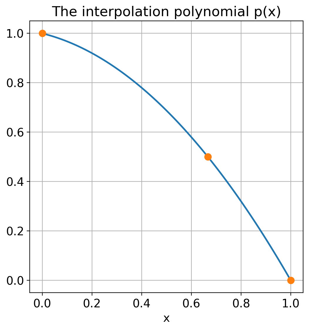
x = np.linspace(0, 1, 101)  # The x-values in which the polynomial is evaluated
p = newton_interpolation(F, xdata, x)
plt.plot(x, p)  # Plot the polynomial
plt.plot(xdata, ydata, "o")  # Plot the interpolation points
plt.title("The interpolation polynomial p(x)")
plt.grid(True)
plt.xlabel("x");

The table of divided differences:
 [[ 1.   -0.75 -0.75]
 [ 0.5  -1.5   0.  ]
 [ 0.    0.    0.  ]]

../_images/1f3c7ee1fd9193a70395863a233a482bcd0afced6443749c2b076696cfb964a4.png

Polynomial interpolation: Newton interpolation

Contents

73. Polynomial interpolation: Newton interpolation#

73.1. Newton interpolation#

73.2. Implementation#