Computers, Waves, Simulations

The Spectral Element Method - Interpolation with Lagrange Polynomials

43. The Spectral Element Method - Interpolation with Lagrange Polynomials

This notebook covers the following aspects:

• Define Lagrange polynomials

• Define a function to initialize and calculate Lagrange polynomial for order N

• Interpolation of a function using GLL collocation points

43.1. Basics

We can approximate an arbitrary function \(f(x)\) using the interpolation with Lagrange polynomials \(l_i\) at given collacation points \(x_i\), i.e.

\begin{eqnarray*} f(x) = \sum f(x_i) \cdot l_i(x). \end{eqnarray*}

The Lagrange polynomials at \(x\) are defined as follows:

\[ \ell_i^{(N)} (x) \ := \ \prod_{k = 1, \ k \neq i}^{N+1} \frac{x - x_k}{x_i-x_k}, \qquad i = 1, 2, \dotsc , N + 1 \]

They are implemented in Python with the following code:

import matplotlib.pyplot as plt
import numpy as np
from gll import gll

# Prettier plots.
plt.style.use("ggplot")

def lagrange(N, i, x, xi):
    """
    Function to calculate  Lagrange polynomial for order N
    and polynomial i [0, N] at location x at given collocation points xi
    (not necessarily the GLL-points)
    """
    fac = 1
    for j in range(-1, N):
        if j != i:
            fac = fac * ((x - xi[j + 1]) / (xi[i + 1] - xi[j + 1]))
    return fac

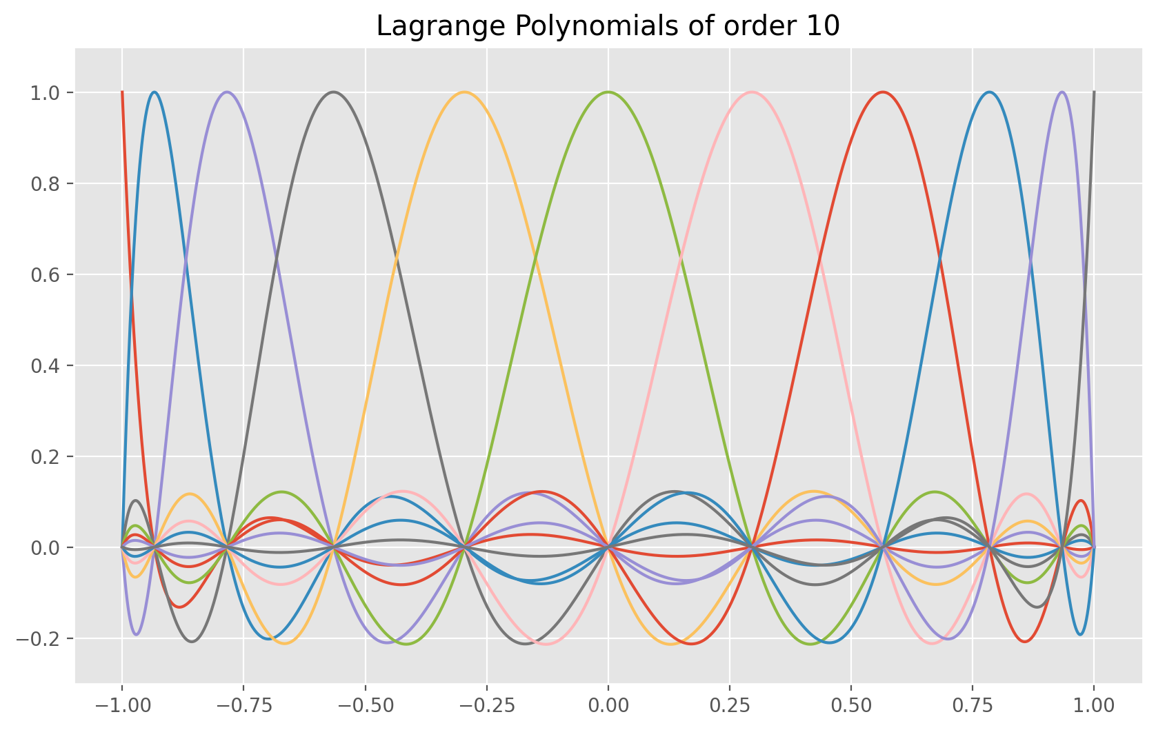
N = 10  # N_max = 12
x = np.linspace(-1, 1, 1000)
xi, _ = gll(N)

# -------------------------------
plt.figure(figsize=(10, 6))
for _i in range(-1, N):
    plt.plot(x, lagrange(N, _i, x, xi))
plt.ylim(-0.3, 1.1)
plt.title("Lagrange Polynomials of order %i" % N)
plt.show()

43.2. Lagrange Interpolation

• Use the gll() routine to determine the collocation points for a given order \(N\) in the interval \([-1,1]\).

• Define an arbitrary function \(f(x)\) and use the function lagrange(N,i,x,x_i) to get the \(i\)-th Lagrange polynomials of order N at the point x.

• Calculate the interpolating function to \(f(x)\).

• Show that the interpolation is exact at the collocation points.

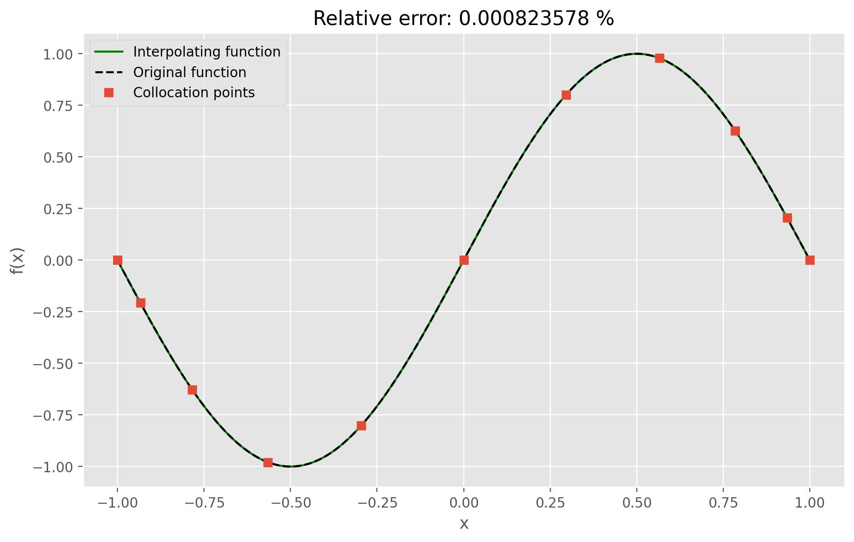
• Compare the original function \(f(x)\) and the interpolating function on a finely spaced grid. Vary the order of the interpolating polynomials and calculate the error as a function of order.

# Lagrange Interpolation
# ----------------------------------------------------------------
# Initialize space in the interval [-1, 1] for plotting the original and interpolated function
nx = 1000
x = np.linspace(-1, 1, nx)

# Define an arbitrary function you want to interpolate (change it!)
f = np.sin(np.pi * x)

# Give order of Lagrange polynomial
N = 10

# Get collocation points xi from gll routine (worth having a look)
[xi, w] = gll(N)
fi = np.interp(xi, x, f)

# Initialize Lagrange polynomials on the defined grid
lp = np.zeros((N + 1, len(x)))
for i in range(0, len(x)):
    for j in range(-1, N):
        lp[j + 1, i] = lagrange(N, j, x[i], xi)

######################################################
# Calculate interpolating polynomials by multiplying
# Lagrange polynomials with function values at xi
s = x * 0
for j in range(0, N + 1):
    s = s + lp[j, :] * fi[j]
#
######################################################

# Calculate error of original and interpolated function
error = np.sum(np.abs(f - s)) / np.sum(np.abs(f)) * 100

# -------------------
# Plot results
plt.figure(figsize=(10, 6))
plt.plot(x, s, "g-", label="Interpolating function")
plt.plot(x, f, "k--", label="Original function")
plt.plot(xi, fi, "s", label="Collocation points")
plt.title("Relative error: %g %%" % error)
plt.xlabel("x")
plt.ylabel("f(x)")

plt.legend(loc="upper left")
plt.show()