Computers, Waves, Simulations

Finite-Difference Method - Second Derivative

28. Second Derivative

This exercise covers the following aspects:

• Initializing a Gaussian test function

• Calculation of numerical second derivative with 3-point operator

• Accuracy improvement of numerical derivative with 5-point operator

Note:

• Loop boundaries changed for 5-point operator, May 2020

import matplotlib.pyplot as plt
import numpy as np

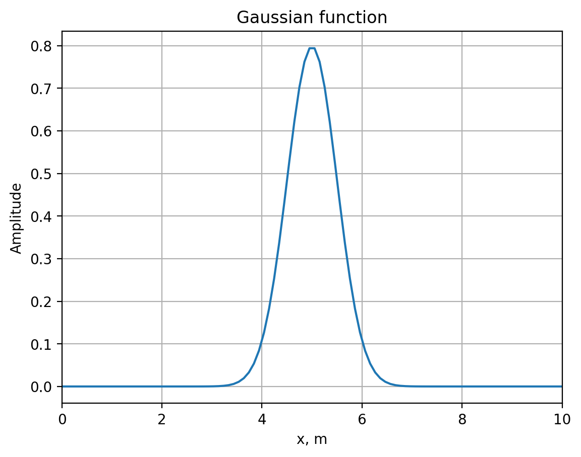
We initialize a Gaussian function

\begin{equation} f(x)=\dfrac{1}{\sqrt{2 \pi a}}e^{-\dfrac{(x-x_0)^2}{2a}} \end{equation}

Note that this specific definition is a \(\delta-\)generating function. This means that \(\int{f(x) dx}=1\) and in the limit \(a\rightarrow0\) the function f(x) converges to a \(\delta-\)function.

# Initialization
xmax = 10.0  # physical domain (m)
nx = 100  # number of space samples
a = 0.25  # exponent of Gaussian function
dx = xmax / (nx - 1)  # Grid spacing dx (m)
x0 = xmax / 2  # Center of Gaussian function x0 (m)

x = np.linspace(0, xmax, nx)  # defining space variable

# Initialization of Gaussian function
f = (1.0 / np.sqrt(2 * np.pi * a)) * np.exp(-(((x - x0) ** 2) / (2 * a)))

# Plotting of gaussian
plt.figure()
plt.plot(x, f)
plt.title("Gaussian function")
plt.xlabel("x, m")
plt.ylabel("Amplitude")
plt.xlim((0, xmax))
plt.grid()

Now let us calculate the second derivative using the finite-difference operator with three points

\begin{equation} f^{\prime\prime}_{\text{num}}\left(x\right)= \dfrac{f\left(x+\mathrm{d}x\right)-2f\left(x\right)+f\left(x-\mathrm{d}x\right)} \end{equation}

and compare it with the analytical solution \begin{equation} f^{\prime\prime}\left(x\right)= \dfrac{1}{\sqrt{2\pi a}} \left(\dfrac{\left(x-x_{0}\right)^2}{a^2}-\dfrac{1}{a}\right) \ \exp\left(-\dfrac{(x-x_0)^2}{2a}\right) \end{equation}

# Second derivative with three-point operator

# Initiation of numerical and analytical derivatives
nder3 = np.zeros(nx)  # numerical derivative
ader = np.zeros(nx)  # analytical derivative

# Numerical second derivative of the given function
for i in range(1, nx - 1):
    nder3[i] = (f[i + 1] - 2 * f[i] + f[i - 1]) / (dx**2)

# Analytical second derivative of the Gaissian function
ader = (
    1.0
    / np.sqrt(2 * np.pi * a)
    * ((x - x0) ** 2 / a**2 - 1 / a)
    * np.exp(-1 / (2 * a) * (x - x0) ** 2)
)
# Exclude boundaries
ader[0] = 0.0
ader[nx - 1] = 0.0

# Calculate rms error of numerical derivative
rms = np.sqrt(np.mean((nder3 - ader) ** 2))

plt.figure()
plt.plot(x, nder3, label="Numerical Derivative, 3 points", lw=2, color="violet")
plt.plot(x, ader, label="Analytical Derivative", lw=2, ls="--")
plt.plot(x, nder3 - ader, label="Difference", lw=2, ls=":")
plt.title("Second derivative, Err (rms) = %.6f " % (rms))
plt.xlabel("x, m")
plt.ylabel("Amplitude")
plt.legend(loc="lower left")
plt.grid()

In the cell below calculation of the first derivative with four points is provided with the following weights:

\begin{equation} f^{\prime\prime}\left(x\right)= \dfrac{-\dfrac{1}{12}f\left(x-2\mathrm{d}x\right)+ \dfrac{4}{3}f\left(x-\mathrm{d}x\right)- \dfrac{5}{2}f\left(x\right)+ \dfrac{4}{3}f\left(x+\mathrm{d}x\right)- \dfrac{1}{12}f\left(x+2\mathrm{d}x\right)} \end{equation}

# First derivative with four points

# Initialisation of derivative
nder5 = np.zeros(nx)

# Calculation of 2nd derivative
for i in range(2, nx - 2):
    nder5[i] = (
        -1.0 / 12 * f[i - 2]
        + 4.0 / 3 * f[i - 1]
        - 5.0 / 2 * f[i]
        + 4.0 / 3 * f[i + 1]
        - 1.0 / 12 * f[i + 2]
    ) / dx**2

# Exclude boundaries
ader[1] = 0.0
ader[nx - 2] = 0.0

# Calculate rms error of numerical derivative
rms = rms * 0
rms = np.sqrt(np.mean((nder5 - ader) ** 2))

plt.figure()
plt.plot(x, nder5, label="Numerical Derivative, 5 points", lw=2, color="violet")
plt.plot(x, ader, label="Analytical Derivative", lw=2, ls="--")
plt.plot(x, nder5 - ader, label="Difference", lw=2, ls=":")
plt.title("Second derivative, Err (rms) = %.6f " % (rms))
plt.xlabel("x, m")
plt.ylabel("Amplitude")
plt.legend(loc="lower left")
plt.grid()

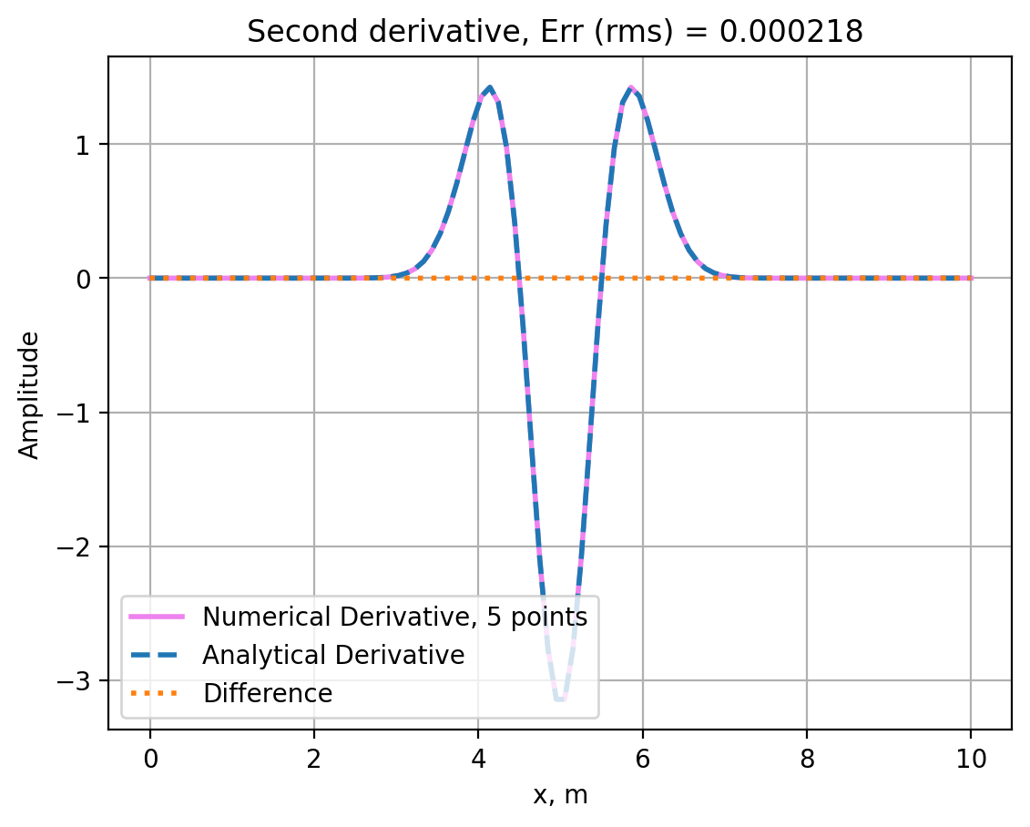
28.1. Conclusions

• 3-point finite-difference approximations can provide estimates of the 2nd derivative of a function

• We can increase the accuracy of the approximation by using further functional values further

• A 5-point operator leads to substantially more accurate results