41. The Finite Element Method - Static Elasticity#
This notebook covers the following aspects:
Define the concept of static elasticity
Solution using finite element scheme
Solution using the finite difference scheme and its comparion with FEM solution
41.1. Basic Equations#
Static elasticity can be considered a particular case derived from the elastic wave equation when the displacement does not depend on time, i.e \(\partial_t^2 u(x,t) = 0\). Under this assumption and departing from the 1D elastic wave equation, the differential equation turns into the Poisson equation
\begin{equation} -\mu \partial_x^2 u = f, \end{equation}
where \(\mu\) is the shear modulus for a homogeneous media, \(u\) is the displacement field, and \(f\) is the external force. The solution for this problems is found after bringing this equation into its weak form, applying the free boundary condition, and using the Galerkin principle with a suitable basis. Then, the displacement defined in a discrete set of points \(x_i\) is given as the solution of a system of N equations, with
\begin{equation} \mathbf{u} = (\mathbf{K}^{T})^{-1} \mathbf{f} \end{equation}
where \(\mathbf{K}\) is the stiffness matrix. For an elastic physical system with constant shear modulus \(\mu\) and uniform element size \(h\), it is given as
\begin{equation} K_{ij} = \frac{\mu}{h} \begin{pmatrix} 1 & -1 & & & \ -1 & 2 & -1 & & \ & & \ddots & & \ & & -1 & 2 & -1 \ & & & -1 & 1 \end{pmatrix} \end{equation}
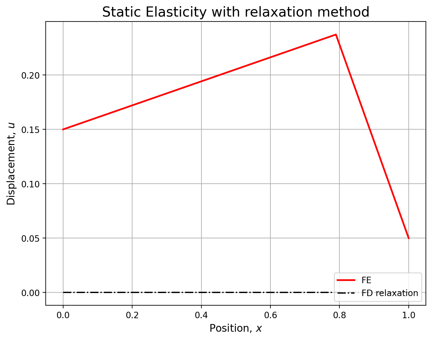
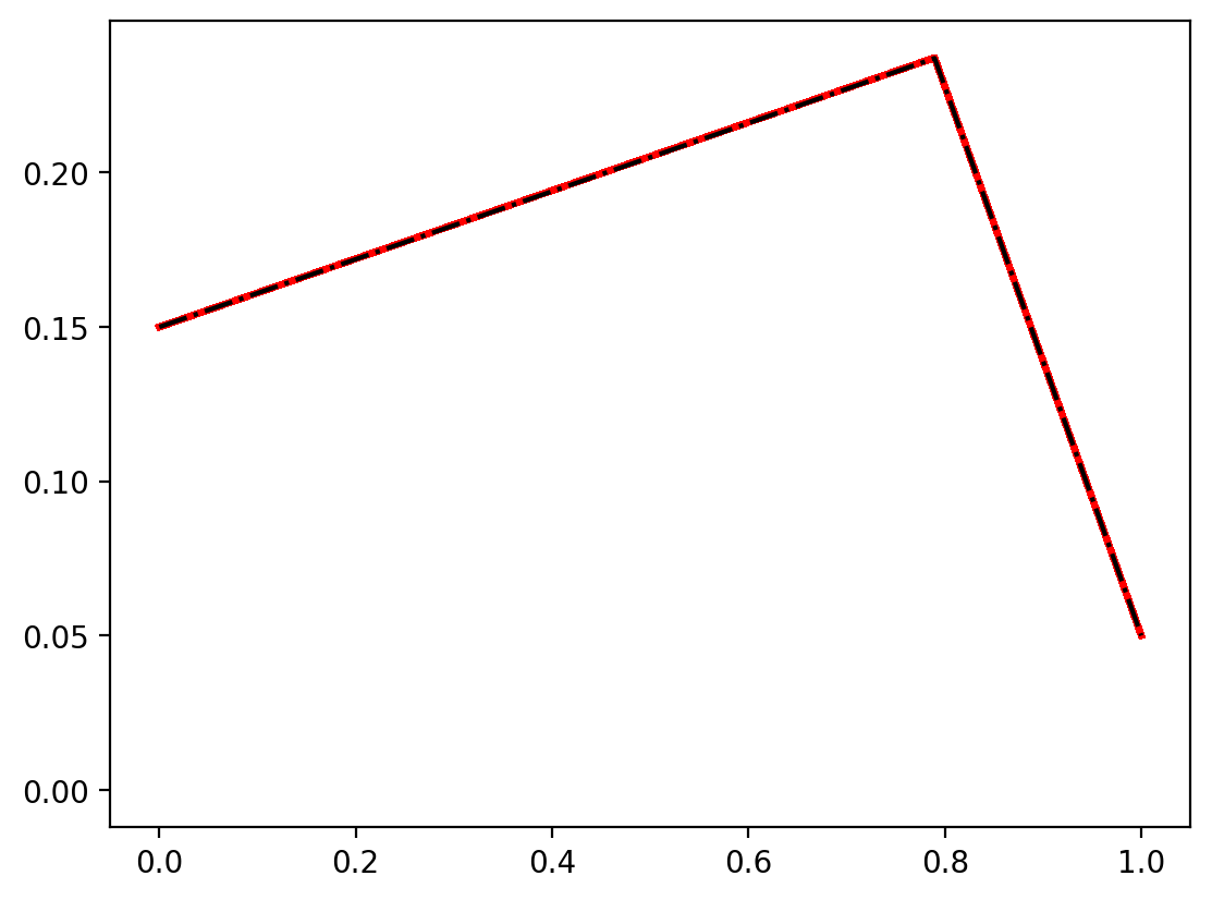
The purpose of this notebook is to illustrate how the problem of static elasticity is solved with the finite- element method. We also compare the solution using finite - differences, the so-called relaxation method given by (derivation in the book):
\begin{equation} u_{i}^{k+1} = \dfrac{u_{i+1}^{k} + u_{i-1}^{k}}{2} + \dfrac{h^2}{2 \mu}f_i \end{equation}
import matplotlib.pyplot as plt
import numpy as np
# matplotlib.use("nbagg")
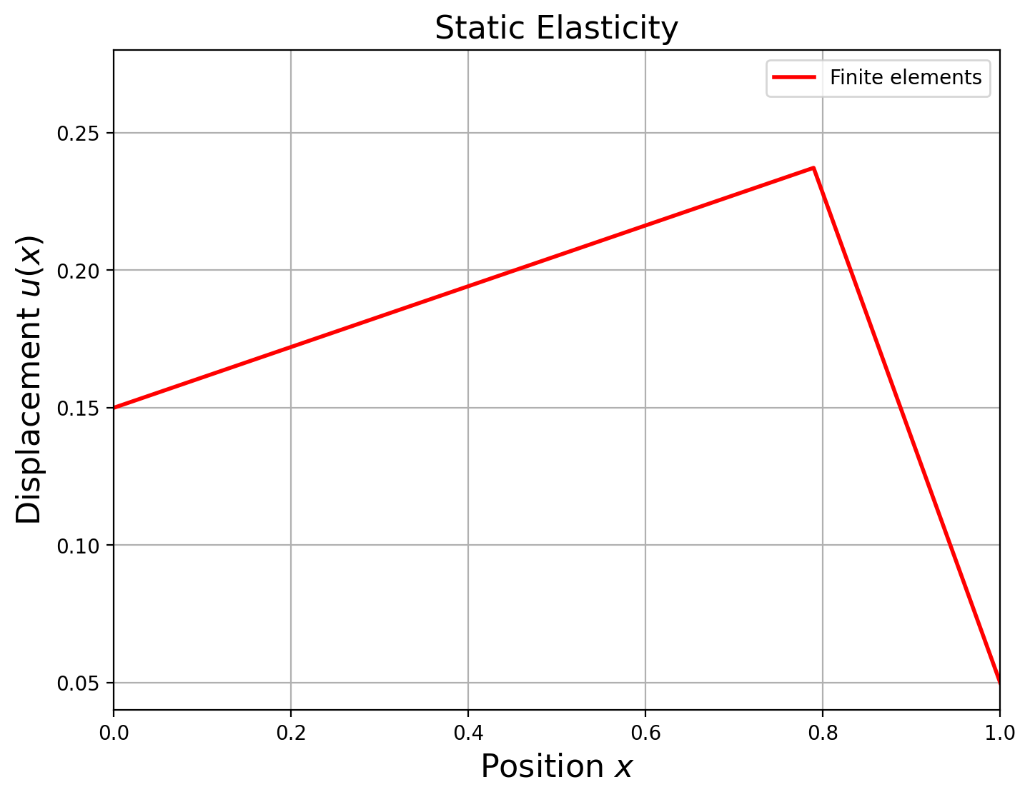
41.1.1. 1. Finite - Element solution#
# ---------------------------------------------------------------
# Initialization of setup
# ---------------------------------------------------------------
nx = 20  # Number of element boundary points
u = np.zeros(nx)  # Solution vector
f = np.zeros(nx)  # Source vector
mu = 1  # Constant shear modulus

# Element boundary points
x = np.linspace(0, 1, nx)  # x in [0,1]
h = x[2] - x[1]  # Constant element size

# ---------------------------------------------------------------
# Assemble stiffness matrix K_ij
# ---------------------------------------------------------------
K = np.zeros((nx, nx))
for i in range(1, nx - 1):
    for j in range(1, nx - 1):
        if i == j:
            K[i, j] = 2 * mu / h
        elif i == j + 1:
            K[i, j] = -mu / h
        elif i + 1 == j:
            K[i, j] = -mu / h
        else:
            K[i, j] = 0

# ---------------------------------------------------------------
# Souce term is a spike at i = 3*nx/4
f[int(3 * nx / 4)] = 1

# Boundary condition at x = 0
u[0] = 0.15
f[1] = u[0] / h

# Boundary condition at x = 1
u[nx - 1] = 0.05
f[nx - 2] = u[nx - 1] / h

# ---------------------------------------------------------------
# Finite element solution
# ---------------------------------------------------------------
u[1 : nx - 1] = np.linalg.inv(K[1 : nx - 1, 1 : nx - 1]) @ np.transpose(f[1 : nx - 1])

# ---------------------------------------------------------------
# Plotting section
# ---------------------------------------------------------------
plt.figure(figsize=(8, 6))

xfe = u
plt.plot(x, xfe, color="r", lw=2, label="Finite elements")
plt.title("Static Elasticity", size=16)
plt.ylabel("Displacement $u(x)$", size=16)
plt.xlabel("Position $x$", size=16)
plt.axis([0, 1, 0.04, 0.28])
plt.legend()
plt.grid(True)
plt.show()
41.1.2. 2. Finite - Difference solution#
# Poisson's equation with relaxation method
# ---------------------------------------------------------------
nt = 500  # Number of iterations
iplot = 2  # Snapshot frequency

# non-zero boundary conditions
u = np.zeros(nx)  # set u to zero
du = np.zeros(nx)  # du/dx
f = np.zeros(nx)  # forcing

f[int(3 * nx / 4)] = 1.0 / h

xfd = np.arange(0, nx) * h

# ---------------------------------------------------------------
# Initialize animated plot
# ---------------------------------------------------------------
plt.figure(figsize=(8, 6))

line1 = plt.plot(x, xfe, color="r", lw=2, label="FE")
line2 = plt.plot(xfd, u, color="k", ls="-.", label="FD relaxation")
plt.title("Static Elasticity with relaxation method", size=16)
plt.ylabel("Displacement, $u$", size=12)
plt.xlabel("Position, $x$", size=12)
plt.legend(loc=4)
plt.grid(True)

plt.ion()  # set interective mode
plt.show()
# ---------------------------------------------------------------
# Initialize boundaries for first time step
u[0] = 0.15  # Boundary condition at x=0
u[nx - 1] = 0.05  # Boundary condition at x=1

for it in range(nt):
    # Calculate the average of u (omit boundaries)
    for i in range(1, nx - 1):
        du[i] = u[i + 1] + u[i - 1]
    u = 0.5 * (f * h**2 / mu + du)
    u[0] = 0.15  # Boundary condition at x=0
    u[nx - 1] = 0.05  # Boundary condition at x=1
    fd = u

    # --------------------------------------
    # Animation plot. Display both solutions
    if not it % iplot:
        for l in line2:
            l.remove()
            del l
        line1 = plt.plot(x, xfe, color="r", lw=2)
        line2 = plt.plot(xfd, fd, color="k", ls="-.")
        plt.gcf().canvas.draw()