37. The Pseudo-Spectral Method - Numerical Derivatives based on a Derivative Matrix#
This notebook covers the following aspects:
Calculating a derivative using the differentation theorem of the Fourier Transform
Define a function that initializes the Chebyshev derivative matrix \(D_{ij}\) for a Gaussian function
Compare with analytical solution
37.1. Basic Equations#
Calculating a derivative using the differentation theorem of the Fourier Transform is in the mathematical sense a convolution of the function \(f(x)\) with \(ik\), where \(k\) is the wavenumber and \(i\) the imaginary unit. This can also be formulated as a matrix-vector product involving so-called Toeplitz matrices. An elegant (but inefficient) way of performing a derivative operation on a space-dependent function described on the Chebyshev collocation points is by defining a derivative matrix \(D_{ij}\)
where \(N+1\) is the number of Chebyshev collocation points \( \ x_i = cos(i\pi / N)\), \( \ i=0,...,N\) and the \(c_i\) are given as
This differentiation matrix allows us to write the derivative of the function \(f_i = f(x_i)\) (possibly depending on time) simply as
where the right-hand side is a matrix-vector product, and the Einstein summation convention applies.
import warnings

import matplotlib
import matplotlib.pyplot as plt
import numpy as np
from matplotlib import gridspec, use
# matplotlib.use("nbagg")
warnings.filterwarnings("ignore")
# Function for setting up the Chebyshev derivative matrix D_ij


def get_cheby_matrix(nx):
    cx = np.zeros(nx + 1)
    x = np.zeros(nx + 1)
    for ix in range(0, nx + 1):
        x[ix] = np.cos(np.pi * ix / nx)

    cx[0] = 2.0
    cx[nx] = 2.0
    cx[1:nx] = 1.0

    D = np.zeros((nx + 1, nx + 1))
    for i in range(0, nx + 1):
        for j in range(0, nx + 1):
            if i == j and i != 0 and i != nx:
                D[i, i] = -x[i] / (2.0 * (1.0 - x[i] * x[i]))
            else:
                D[i, j] = (cx[i] * (-1.0) ** (i + j)) / (cx[j] * (x[i] - x[j]))

    D[0, 0] = (2.0 * nx**2 + 1.0) / 6.0
    D[nx, nx] = -D[0, 0]
    return D
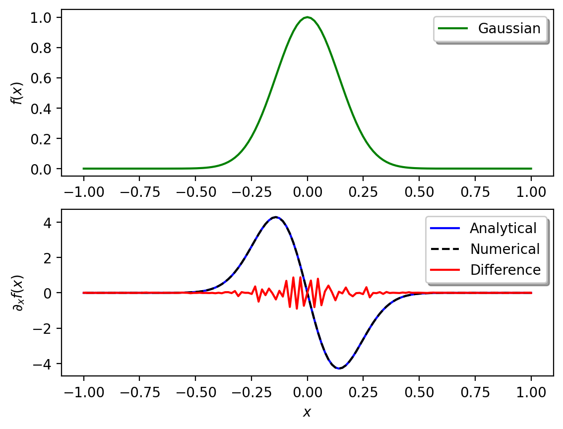
The following cels defines an arbitrary function (e.g. a Gaussian) and initialize its analytical derivative on the Chebyshev collocation points and calculates the numerical derivative and the difference to the analytical solution.
# Initialize arbitrary test function on Chebyshev collocation points
nx = 200  # Number of grid points - can be modified
x = np.zeros(nx + 1)
for ix in range(0, nx + 1):
    x[ix] = np.cos(ix * np.pi / nx)
dxmin = min(abs(np.diff(x)))
dxmax = max(abs(np.diff(x)))

# Function example: Gaussian
# Width of Gaussian
s = 0.2
# Gaussian function (modify!)
f = np.exp(-1 / s**2 * x**2)

# Analytical derivative
df_ana = -2 / s**2 * x * np.exp(-1 / s**2 * x**2)

# Initialize differentiation matrix
D = get_cheby_matrix(nx)

# Calculate numerical derivative using differentiation matrix D_{ij}
df_num = D @ f

# To make the error visible, it is multiply by 10^12
df_err = 1e12 * (df_ana - df_num)

# Calculate error between analytical and numerical solution
err = np.sum((df_num - df_ana) ** 2) / np.sum(df_ana**2) * 100
print("Error: %s" % err)
Error: 1.8942124148740918e-24
# ----------------------------------------------------------------
# Plot analytical and numerical derivatives
# ---------------------------------------------------------------

plt.subplot(2, 1, 1)
plt.plot(x, f, "g", lw=1.5, label="Gaussian")
plt.legend(loc="upper right", shadow=True)
plt.xlabel("$x$")
plt.ylabel("$f(x)$")

plt.subplot(2, 1, 2)
plt.plot(x, df_ana, "b", lw=1.5, label="Analytical")
plt.plot(x, df_num, "k--", lw=1.5, label="Numerical")
plt.plot(x, df_err, "r", lw=1.5, label="Difference")
plt.legend(loc="upper right", shadow=True)
plt.xlabel("$x$")
plt.ylabel(r"$\partial_x f(x)$")

plt.show()